Computer Music Composition and Production

Programming Examples

Programming examples for the class
Music 215A: Computer Music Composition and Production - Winter 2019
University of California, Irvine

This page contains examples and explanations of techniques of computer music programming using Max.

The examples were written for use by students in the Computer Music Composition and Production course at UCI, and are made available on the WWW for all interested Max/MSP/Jitter users and instructors. If you use the text or examples provided here, please give due credit to the author, Christopher Dobrian.

The largest single collection of Max examples is the Max Cookbook. You can find specific examples there by title or by keyword search.

While not specifically intended to teach Max programming, each chapter of Christopher Dobrian's algorithmic composition blog contains a Max program demonstrating the chapter's topic, many of which address fundamental concepts in programming algorithmic music and media composition.

Please note that all the examples from the years prior to 2009 are designed for versions of Max prior to Max 5. Therefore, when opened in Max 5 or 6 they may not appear quite as they were originally designed (and as they are depicted), and they may employ some techniques that seem antiquated or obsolete due to new features introduced in Max 5 or Max 6. However, they should all still work correctly.

[Each image below is linked to a file of JSON code containing the actual Max patch.
Right-click on an image to download the .maxpat file directly to disk, which you can then open in Max.]

Max Examples

Examples will be added after each class session.

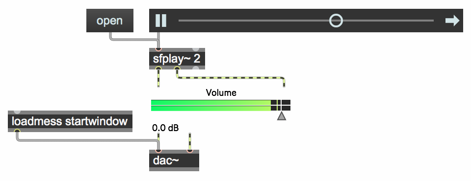
Example 1: Simple audio file player

This shows a simple replication of a basic audio file playing program such as QuickTime Player. The core of the program is the sfplay~ object. The object expects to receive an open message, which presents the user with a dialog for selecting a sound file in to open. In this patch, we use a textbutton object to send the message open when the user clicks on the button. The output of sfplay~ goes through a live.gain~ object to allow the user control of the volume before it goes on to the dac~ object, which sends the sound signal to the computer's speakers (or whatever audio interface is currently chosen in Max's Audio Status window). The loadmess object sends the message startwindow to the dac~ object to turn audio processing on as soon as the patch is opened. Basic playback control—start/stop, looping on/off—is done with a playbar object, which sends control messages to sfplay~. Another way to control sfplay~ would be to use the basic messages it understands: 1, 0, pause, resume, loop 1, loop 0, etc. That more basic control of sfplay~ is demonstrated in "Open a sound file and play it" from a previous year's class.

A few other examples from past classes relevant to the task of soundfile playback are:
"Preload and play sound cues"
"Trigger sound cues from the computer keyboard"
"Trigger sound cues with the mouse or from the computer keyboard"
"Using presentation mode"

Example 2: Play a sound file with vibrato

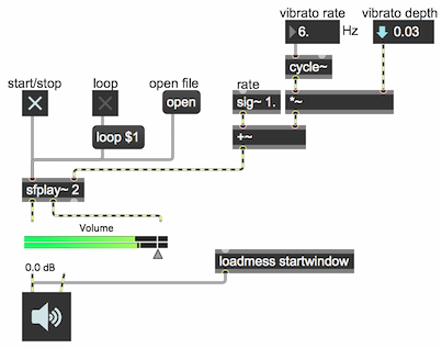
To impose a vibrato (a periodic fluctuation of frequency) on the playback of a sound file, you can use a low-frequency oscillator (a cycle~ object) to modulate the playback speed of the file. The right inlet of the sfplay~ object controls the playback speed with a rate factor. A value of 1 is normal speed (the default), 2.0 is double speed, 0.5 is half speed, etc. The speed can be supplied as a constant number (float) or with a continuous signal. So, you can supply a constant signal of 1 with a sig~ 1 object, and add to that a small offset up and down by means of a low-frequency low-amplitude sinusoidal oscillator (cycle~).

Example 3: Play a sound from RAM with vibrato

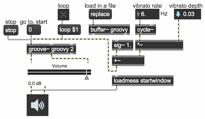
In the groove~ object, you specify the rate of playback of a buffer~ by means of a signal in the left inlet of groove~. Normal playback speed is achieved with a signal value of 1. As shown in Example 2 above, you can create a vibrato by modulating that signal with a low-frequency oscillator.

Example 4: How the adsr~ object works

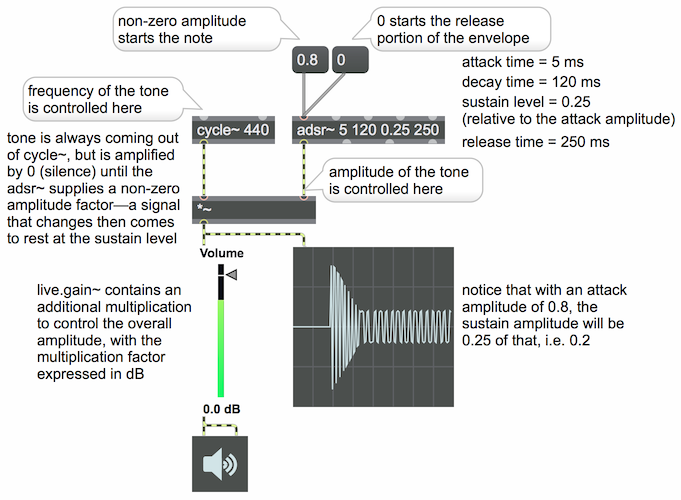
The adsr~ object provides a signal in the shape of an ADSR envelope (attack, decay, sustain, release) commonly used in synthesizer design. You specify an attack time in ms (time to get from 0 amplitude to peak amplitude), a decay time in ms (time to settle to the sustain level), a sustain level (an amplitude factor, not a ms time), and a release time in ms (time to return to 0). Those values can all be supplied as initializing arguments, and/or as floats or signals in the second, third, fourth, and fifth inlets. (Although signals are allowed, it's more common to use float values.) When a non-zero value is received in the left inlet, that determines the peak amplitude of the attack; the attack and decay portions of the envelope are completed in the designated amounts of time, then the output signal stays at the sustain level until a 0 value is received in the left inlet, at which point the release portion of the envelope is enacted.

An ADSR envelope can be used to control any aspect of a sound—amplitude, filter cutoff frequency, modulation amount, etc. In this example, we use it to control the amplitude of a tone, by sending the output of adsr~ to one of the inlets of *~.

Example 5: Play eight samples automatically at a constant rate

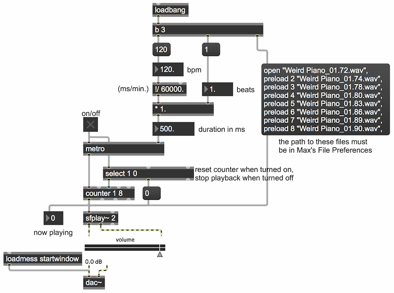
This patch shows how to load multiple sound files as sound "cues" in the sfplay~ object, then how to use the metro and counter objects to step through them one-by-one automatically at a constant rate. The sound files must be in the file search path, which is to say that the folder that contains them must be listed in Max's File Preferences... window, accessed in the Options menu. Whenever the metro is started, we first also send a bang in the middle inlet of the counter, to reset it to its minimum value. And whenever the metro is stopped, we also send a 0 to sfplay~ to stop whatever sound cue is currently playing. The rate at which the metro runs is calculated based on some metronomic tempo and the number of beats we want to use as the note rate. When the patch is started, we use loadbang to initialize the tempo to 120 bpm and the duration of each sound cue to be 1 beat, which results in a metro interval of 500 ms; and we preload the eight sound cues into sfplay~, and we turn on the dac~. That way, the program is totally ready to run when the patch is loaded.

Example 6: Generate a window function to use as an amplitude envelope

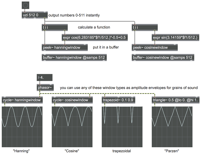
To play short grains of sound, especially ones randomly chosen from a sound file, it's usually necessary to impose some sort of "window"—an amplitude envelope—to taper the ends of the grain in order to avoid clicks. This patch shows how to generate four types of window function, and read through them with a phasor.

One way to generate a window is to fill a buffer~ with a shape and then read through that buffer. The top part of the patch shows that method. We create a buffer~ of 512 samples, and use the peek~ object to put numbers in the buffer~. The uzi 512 0 object generates numbers 0-511 in an instant (i.e., as quickly as possible); those numbers are used in 512 iterations of a math expression in the expr object, and the results are stored in the 512 locations in the buffer~. Click on the button to trigger the uzi, then double-click on the buffer~ object to see its contents.

We chose 512 as the number of samples because a cycle~ object can refer to 512 samples of a buffer~ and use that shape as its waveform instead of its default cosine wave. We can read through one cycle of that waveform at any frequency. By specifying no frequency for cycle~, it's at 0 Hz by default, and we can then read through it with a phasor~— a signal going linearly from 0 to 1—going into the right (phase offset) inlet of the cycle~. The bottom part of the patch also demonstrates the use of the trapezoid~ and triangle~ objects, which output those shapes when driven by a phasor~.

Example 7: Play a stream of random grains from a sound file

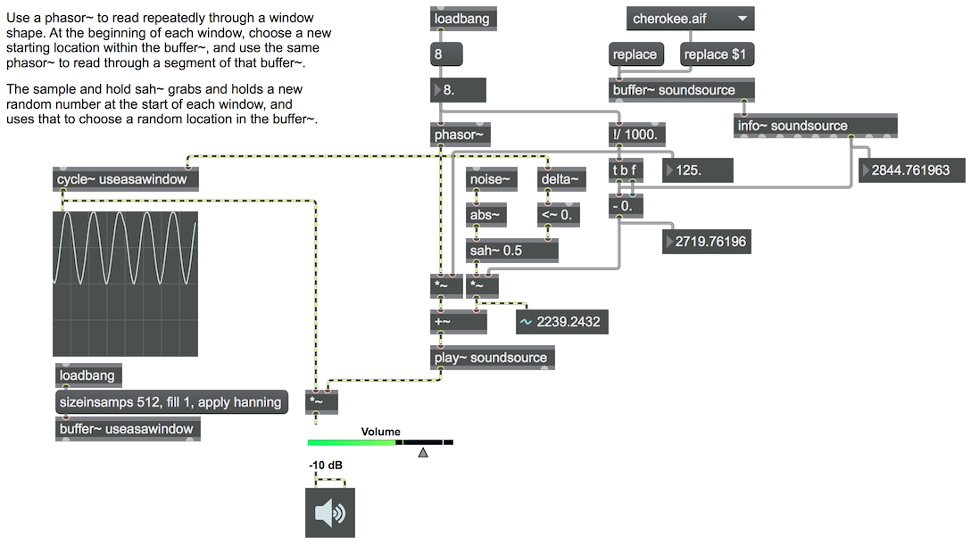
This patch demonstrates a method for playing a stream of sound grains randomly chosen from a sound file.

We first load a sound file into a buffer~. When you use the replace message to load the file, the buffer~ will be resized to the size of the sound file, and buffer~ will send a bang out of its right outlet when it has finished loading the file. The bang can be used to trigger an info~ object, which will report information about the sound file. The info we care about in this case is the file's duration; that duration, in milliseconds, will tell us the range of numbers we can use to specify a grain segment we want to play.

The phasor~ object is used here to read through a segment of the sound, and also to read through the windowing function contained in the buffer~ useasawindow, which we have filled with a Hann (a.k.a. Hanning) window function. That window shape will be used to taper the amplitude of the grain of sound at each end, thus avoiding clicks.

Since we know the frequency of the phasor~ in cycles per second, we can easily calculate its period in ms (1000/frequency), giving us the duration of each grain. At just the precise moment when each new grain starts—when the window function has tapered the sound's amplitude down to 0—we choose a new starting location in the buffer~. We can detect when the phasor~ starts a new cycle by checking its change with the delta~ object. At the moment when the phasor~ leaps from 1 back to 0, the change will suddenly be negative, causing a 1 value to come out of the <~ 0 object. That will trigger the sah~ (sample and hold) object to grab a random value from the noise~ object (the absolute value of which will be between 0 and 1). We multiply that by the duration of the buffer~, and use the result to set a new random starting point in the buffer~. From that point, we read through the next grain of sound (the duration of which we calculated using the period of the phasor~). Because we choose the new location at the very beginning of the phasor~'s cycle, the amplitude will be 0 at that moment, so there will be no discontinuty in the sound. The result is a continuous stream of randomly chosen bits of sound, at a constant rate, windowed by the Hanning function.

This page was last modified February 19, 2019.
Christopher Dobrian, dobrian@uci.edu