Programming examples for the class
Music 215B: Computer Music Programming - Winter 2016
University of California, Irvine
This page contains examples and explanations of techniques of computer music programming using Max.
The examples were written for use by students in the Computer Music Programming course at UCI, and are made available on the WWW for all interested Max/MSP/Jitter users and instructors. If you use the text or examples provided here, please give due credit to the author, Christopher Dobrian.
Examples from previous classes are also available on the Web:
Examples from Music 152/215, winter 2015
Examples from Music 152/215, spring 2014
Examples from Music 147, spring 2014
Examples from Music 152/215, spring 2013
Examples from Music 215, spring 2012
Examples from Music 152/215, winter 2012
Examples from Music 152/215, winter 2011
Examples from Music 152/215, spring 2010
Examples from Music 152/215, spring 2009
Examples from Music 152/215, spring 2007
Examples from Music 147, winter 2007
Examples from Music 152/215, spring 2006
Examples from COSMOS, summer 2005
Examples from Music 152/215, spring 2005
MSP examples from Music 152, spring 2004
Jitter examples from Music 152, spring 2004
While not specifically intended to teach Max programming, each chapter of Christopher Dobrian's algorithmic composition blog contains a Max program demonstrating the chapter's topic, many of which address fundamental concepts in programming algorithmic music and media composition.
Please note that all the examples from the years prior to 2009 are designed for versions of Max prior to Max 5. Therefore, when opened in Max 5 or 6 they may not appear quite as they were originally designed (and as they are depicted), and they may employ some techniques that seem antiquated or obsolete due to new features introduced in Max 5 or Max 6. However, they should all still work correctly.
[Each image below is linked to a file of JSON code containing the actual Max patch.
Right-click on an image to download the .maxpat file directly to disk, which you can then open in Max.]
Examples will be added after each class session.
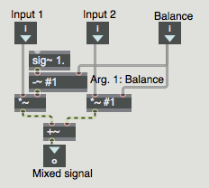
Example 1: A useful subpatch for mixing and balancing two sounds
To mix two sounds together equally, you just add them together. If you know that both sounds will frequently be at or near full amplitude (peak amplitude at or near 1) then you probably want to multiply the result by 0.5 after you add them together, to avoid clipping. However, if you want to mix two sounds unequally, with one sound having a higher gain than the other, a good way to accomplish that is to give one sound a gain between 0 and 1 and give the other sound a gain that's equal to 1 minus that amount. Thus, the sum of the two gain factors will always be 1, so the sum of the sounds will not clip. When sound A has a gain of 1, sound B will have a gain of 0, and vice versa. As one gain goes from 0 to 1, the gain of the other sound will go from 1 to 0, so you can use this method to create a smooth crossfade between two sounds.
Example 2: A useful noisegate (ducker) subpatch for rejecting unwanted sounds
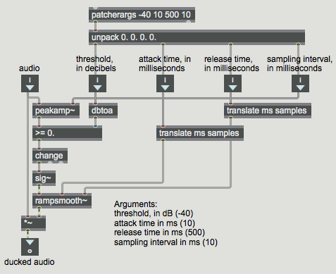
A "ducker" is a system that turns a signal down to 0 when it's below a given threshold. This is also frequently called a "noisegate" in audio engineering, because it acts as a doorway that closes out unwanted low-level ambient noise and lets through only the louder, more desired signal. It's useful for suppressing unwanted low-level audio, such as in a cell phone transmission when the user is not talking, or, more to the point for musical purposes, as in a microphone signal when the musician is not playing.
You can include this subpatch in your MSP audio signal chain somewhere between the sound source (such as adc~) and other processors or analyzers in which you want to suppress ambient noise. The patch allows you to set a threshold, specified in decibels, above which the incoming audio signal will pass unaltered, and below which the signal will get turned down to complete silence. It uses the peakamp~ object to monitor the peak amplitude of the incoming audio signal, to see if the peak is above or below the threshold. (You could make a version of this that uses RMS amplitude instead, with the average~ object instead of peakamp~, but I find that the peak amplitude is a more useful measurement in most situations and using it causes the ducker to be more quickly responsive.) You can set the monitoring interval in milliseconds. The patch also allows the user to set "attack" and "release" times, in milliseconds; the "attack" value determines how quickly the gain will be turned up to unity when the peak amplitude rises above the threshold, and the "release" value determines how quickly the sound will be turned down when its peak amplitude falls below the threshold. The rampsmooth~ object smooths the transitions from 0 to 1 (sound being turned on), and from 1 to 0 (sound being turned off), over the specified amounts of time. Because the rampsmooth~ object expects time to be specified in samples rather than ms (not so intuitive for the user), the translate object is used to convert milliseconds (what the user cares about) into samples (what rampsmooth~ cares about).
The above-mentioned values -- threshold, attack time, release time, and monitoring interval -- can be sent in the inlets. Those values can initially be specified as typed-in arguments in the parent patch, if so desired, thanks to the patcherargs object. If no values are provided explicitly by the user, patcherargs provides useful initial default values: threshold of -40 dB, attack time of 10 ms, release time of 500 ms, and monitoring interval of 10 ms.
Example 3: Subpatch for playing sound cues from sflist~
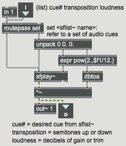
This is a subpatch that can be used for playing sound cues from an sflist~ object. It has one inlet and one outlet, and -- serving the same purpose -- it also has an in object and an out~ object; thus, it can be used either as a normal subpatch or as the content of a poly~ object. It's monophonic, but one could easily adapt it to make a stereo version.
The object that plays the sound cue is sfplay~. Rather than sending 'open' or 'preload' messages to that object, this subpatch assumes that there is an sflist~ object somewhere else that contains the necessary sound cues. So you just refer this sfplay~ object to that sflist~ by sending in the message 'set' followed by the name of the sflist~.
For playing a sound cue, this subpatch expects to get three pieces of information in a single list: the cue number (referring to the sflist~), a number of semitones you'd like to transpose the sample by means of speed change (the transposition can be a fractional number), and the number of decibels of gain or trim you'd like to use to alter the amplitude of the sound. To provide all that information, you send in a three-item list. If you send in a two-item list, the amplitude will stay the same as previously designated (unity gain initially). If you send in just a single number (the cue number), the previous transposition and amplitude will be used.
When multiple copies of this subpatch are used (as in a poly~, for example), each voice of the poly~ could refer to a different sflist~ if so desired, or they could all refer to the same sflist~. This is quite a simple yet versatile patch, because you have easy control of the choice of sample, its transposition, and its amplitude. To stop a sound cue, of course, you just need to send in 0.
Example 4: Six samples at six pitches at six tempi
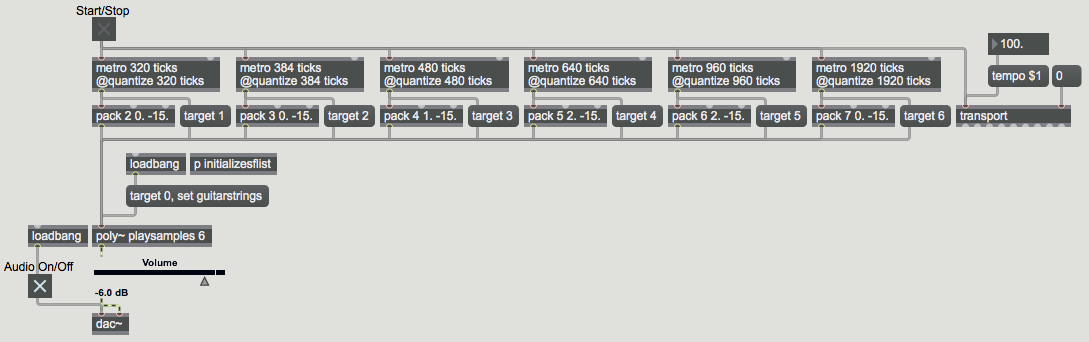
In order for this patch to work properly, you'll need to first download this .zip archive of six short soundfiles, uncompress it, and put the sound files in the Max search path.
You'll also need to download the subpatch for paying sound cues from sflist~ from the previous example. Save it with the name "playsamples.maxpat" in the Max file search path.
Once you have the six soundfiles and the "playsamples" subpatch in the Max file search path, this example patch will work.
This patch plays the six notes of an E major guitar chord at six different tempi, in the ratios 1:2:3:4:5:6. It uses 6 guitar samples (which you'll need to put in the Max file search path), a 6-voice poly~ for playing samples (using the "playsamples" subpatch), and the sflist~ object so that all 6 sfplay~ objects in the poly~ can access the 6 cues.
Example 5: Six upper harmonics of a fundamental
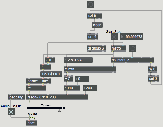
In keeping with the theme of sound patterns based on the number 6, this patch a) uses the urn object to generate a list consisting of a random ordering of the six digits 0 to 5, b) uses a metro to bang a counter six times per second in order to count through that list of digits, c) uses those six digits to produce six frequencies representing harmonics 7 through 12 of a fundamental (110 Hz, initially), and d) uses those frequencies to set the center frequency of a resonant bandpass filter (the reson~ object) to produce six differently filtered noise bursts. Each pattern of six frequencies, played at a rate of six notes per second, is repeated six times, and then a new pattern is selected. (The urn is re-triggered whenever the counter has completed six cycles.)
Example 6: Arpeggiate 16 harmonics of a fundamental
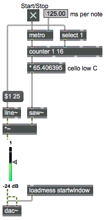
This patch simply arpeggiates the first 16 harmonics of cello low C, so that you can hear the pitches of the harmonic series. You can play them at any rate you want (up to 100 notes per second).
Example 7: Show the sum of harmonically-related sinusoids
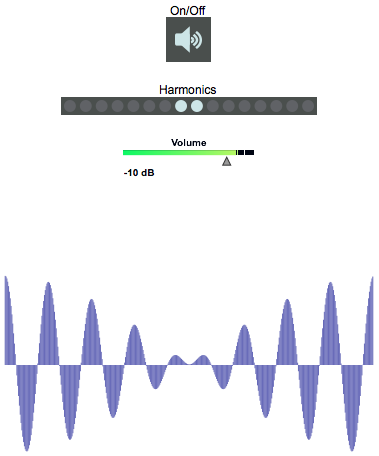
This patch allows you to see and hear the sum of up to 16 harmonically-related sinusoidal tones, mixed with equal amplitudes. The sinusoids are all in cosine phase. (If the phases were different, the sum would look different, but it would sound pretty much the same.) As you add a number of tones together, you'll need to adjust the volume to avoid clipping.
Example 8: Pitch and loudness formulae
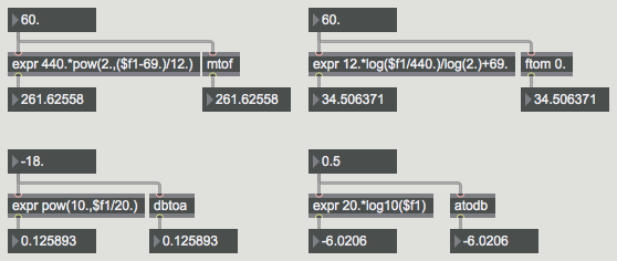
This patch doesn't do anything musical, but it shows the math formulae that underlie the mtof, ftom, atodb, and dbtoa objects.
The base frequency of 440 Hz is defined as the pitch A above middle C, MIDI key number 69. Each semitone up or down is a change by a factor of the 12th root of 2. So, we subtract 69 from any MIDI key number (to find the pitch difference in semitones from A 440) and use that number divided by 12 as the exponent of the base 2, multiplied by the base frequency of 440. For example, Bb above middle C (MIDI 70) has a frequency of 440 times 2 to the (70-69)/12 power. You can verify that this expresson in the expr object yields the same result as the mtof object. For converting frequency to MIDI pitch, we effectively reverse that process, using a logarithm to the base 2. (Because the expr object doesn't have a log2 function, to get log2(x) you have to substitute log(x)/log(2).)
A decibel is a measure of relative value (of power, intensity, etc.), and thus it implies a comparison (specifically, the ratio) of one value to another: the ratio of one value to an established reference value. So, to calculate a value in decibels, you must first find the ratio of that value to some reference value. In computer music, the reference amplitude (let's call it "Aref") is usually 1, so the ratio A/Aref is A/1, which is just A. In dealing with amplitudes, because amplitude squared is proportional to intensity, we effectively need to square the values. To find the number of bels that that represents, you calculate the logarithm to the base 10 of that ratio (in this case, A), and multiply that by 10 (since there are 10 decibels per bel), and then multiply that by 2 because we want the number of decibels represented by the square of A. In short, the formula is: amplitude in decibels is 20 times the log10 of A/Aref. To convert decibels to absolute amplitude, you essentially reverse that process.
Example 9: Linear and exponential
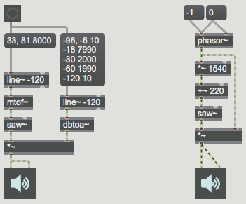
This patch makes a couple of sounds that permit us to compare the sound of linear and exponential changes in pitch and amplitude.
In the left side of the patch, clicking on the button causes a linear change in pitch (which is to say an exponential change in frequency) from low A (MIDI key number 33, 55 Hz fundamental, three ledger lines below the grand staff) to high A (MIDI key number 81, 880 Hz, the ledger line above the grand staff). At the same time, it effects an immediate 10 ms rise in amplitude to -6 dB followed by about an 8-second diminuendo to -18 dB, followed by a much more precipitous dropoff to complete silence in the next four seconds; all these changes are specified linearly in dB, so they cause exponential changes in absolute amplitude.
On the right side of the patch, a phasor~ with a frequency of -1 Hz causes a linear downward ramp from 1 to 0 every second; that ramp is used to control amplitude (from 1 to 0) and frequency (from 1760 Hz to 220 Hz). Linear changes of frequency and amplitude cause a perceptual effect of logarithmic changes (inverse exponential change) in pitch and loudness.
Example 10: 1/4 of a sine wave as a control shape
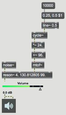
The cycle~ object uses a lookup table of 512 values that make the shape of a single cycle of a cosine wave, and it reads through those repeatedly at whatever rate is specified in its left (frequency) inlet. You can also set the cycle~ to O Hz (its default frequency) and select a point in the cosine waveform with a value (either a signal or a float) from 0 to 1 in the right (phase offset) inlet. Thus, you can get a sinusoidal shaped signal (or any part of one) any time you want by sending the appropriate lookup values in the right inlet of cycle~.
This patch shows an example of using one fourth of a sinusoid to make a control shape. The line~ object sends a signal that goes linearly from 0.25 to 0.5 in 10 seconds. Since that signal is used as the lookup index in the cosine wavetable, cycle~ sends out a signal that goes from 0 to -1 in the shape of the second fourth of the wavetable. That 0 to -1 signal is scaled into the pitch range 96 to 72 (in MIDI-style values), resulting in a 2-octave change in the center frequency of the resonant bandpass filter (reson~) with a slowing curve easing it into the arrival pitch.
Example 11: Linear motion in two voices
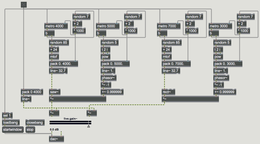
Two oscillators, one in the left channel and one in the right channel, play notes that have a continuously changing frequency, at a continuously changing note rate. Every few seconds (some randomly-chosen number of seconds from 2 to 8) each of the two oscillators gets a new destination frequency and destination note rate, and heads toward those destination values over the next few (randomly-chosen number of) seconds.
You can see a couple of useful Max tricks in the lower left corner of the patch. We use loadbang to turn on audio automatically so that the user doesn't need to think about that. (The 'startwindow' message to dac~ turns on audio locally in that one window, without turning it on in the rest of Max.) We also use a select object (a.k.a. sel) to detect when the toggle is turned on, to make extra sure that audio is on. That's not strictly necessary, and is a little redundant, but it's always possible that audio could get turned on or off in another window somewhere after this patch is opened, so we put this in just in case. The 'startwindow' message turns off audio in other windows, so that you only hear this window. We use pack, line~, and *~ to do a 4-second fade-in/fade-out each time the toggle is turned on or off, just to make the beginning and ending a bit more graceful.
The rest of the patch is the part that makes the sound. There are two soundmaking portions, and they're nearly identical, so let's just look at one of them.
We use a saw~ object to generate a band-limited sawtooth waveform*, like an old-school synthesizer. The sawtooth oscillator gets its frequency from a line~ object (set at 32.7 Hz initially, which is the low C of the piano). The amplitude of the sawtooth is controlled by a phasor~ which is inverted (multiplied by -1) and then pushed back into the positive range (is offset by nearly 1)** so that, instead of ramping from 0 up to 0.999999 then leaping back down to 0, it now leaps up to 0.999999 and ramps back down to 0, making a nice sudden percussive attack and a smooth decay when used as an amplitude envelope. So this phasor~ is actually being used to shape the amplitude of the saw~, in effect playing individual notes of sawtooth sound. The rate of the phasor~ is controlled by a line~ object (set at 1 Hz initially).
The value of those two line~ objects will be continually changing based on the four objects just above them. The frequency of the oscillator is determined the output of the line~, and the destination value of the line~ is determined by a random pitch from piano low C to piano high C. We choose a random MIDI key number from 0 to 84, add 24 to it so that it's now in the range 24 to 108, and then convert that to a frequency using the mtof (MIDI to frequency) object, a simple algebraic equation.*** That frequency destination value gets combined with a ramp time in pack and sent to line~ as a destination value and ramp time pair. The note rate is calculated in a similar manner. We choose a random number 0 to 4, and use that as a power of 2. That is, we use it as the exponent in the pow object, with a base of 2, to calculate 2 to the n power. The result will be 1, 2, 4, 8, or 16 notes per second. That note rate destination value gets combined with a ramp time and sent to line~.
At the top, we have a metro with an initial time interval of 4000 ms (the same as the initial destination time in the pack object). When the metro sends a 'bang', we send a new frequency instruction to line~, as described in the previous paragraph. Then we randomly choose a number from 0 to 6, add 2 to it, and multiply that by 1000, to get a random number of seconds from 2 to 8 (2000 to 8000 ms). We use that time interval to prepare for the ramp time of the next instruction to line~, and to set up the interval for the next scheduled output of the metro. In this way, the ramp time of line~ and the rate of the metro changes to some (usually different) number of seconds with every output. The exact same sort of operation is done with the metro and line~ objects controlling the note rate. The fact that we're using a different metro and a different random object means that the two metros for frequency and note rate are independent and not really in sync, except for the fact that they are always using some whole number of seconds as their interval so they occasionally will coincide recognizably.
The sound generator for the right channel is nearly identical, except that it uses a band-limited square wave oscillator****, rect~, as its sound source, so its sound will be distinguishable from that of the saw~ object. All four metros are initially set to mutually prime time intervals, so that they start out not being in sync with each other. However, because the random objects are choosing from the same relatively small number of time intervals, the sums of their chosen time intervals occasionally match, so that we sometimes get fortuitous coincidence of some aspect of the two sounds. This gives the impression that there is some intentionality or organization, and in fact there is -- the time values were chosen intelligently by the programmer -- just enough to keep the music engaging. Likewise, the limited range of choices for destination note rate (1, 2, 4, 8, or 16 notes per second) causes the tempo of the two note-generators to converge occasionally in interesting ways.
For simplicity, I didn't add in any more complexity that might have made the sounds themselves more interesting, but you can probably imagine some modifications that might make this patch even more sonically/musically interesting: filter envelopes on each note, slow filter sweeps, small delays, echoes, time-varying delays, reverb, etc. Heck, what about dynamics? At present there's no variation in amplitude. Any perceived variation in loudness is really just due to our frequency-dependent perception and cognition. Despite the somewhat annoyingly simplistic sounds, I find that this simple algorithm produces a continuously changing counterpoint that remains interesting, if not expressive, for at least a minute or two.
* A sawtooth wave is described in MSP Tutorial 3. A sawtooth is a waveform that contains all the harmonics of the fundamental frequency, with amplitudes inversely proportional to the harmonic number. The 2nd harmonic has 1/2 the amplitude of the 1st harmonic, the 3rd harmonic has 1/3 the amplitude, etc. So, it's richer and buzzier than a sine tone. The phasor~ object makes a kind of idealized sawtooth shape, which is useful as a control signal, but it's not so great as an audio wave because it has, theoretically, infinite harmonics and can therefore cause aliasing. For that reason, MSP includes an object called saw~ that uses a different formula to calculate a waveform that sounds similar to a sawtooth, but that does not produce harmonics above the Nyquist frequency (half the sampling rate).
** Although it's easy to say that a phasor~ object makes a ramp from 0 to 1, it's more accurate to say that it goes from 0 to almost 1. The output of phasor~ is calculated by continuously interpolating between 0 and 1 based on its rate. It never actually sends out a signal of 1, because at that point it wraps back around to 0. (And depending on how fast it's going, you can't rely on it outputting a true 0 either, since that 0 might fall in between successive samples.) Thus, the actual range of phasor~, based on 32-bit floating point calculations, is 0 to 0.999999.
*** f equals 440 times (2 to the (m-69)/12 power), if you really must know.
**** An ideal square wave produces all the harmonic frequencies of the fundamental in inverse-square proportion to the harmonic number. For example, the 2nd harmonic has 1/4 the amplitude of the 1st harmonic, the 3rd harmonic his 1/9 the amplitude, etc. Thus, it's somewhat less bright and buzzy than a sawtooth wave. Similarly to saw~, the rect~ object uses a different formula to calculate a waveform that sounds similar to a square wave, but that does not produce harmonics that would cause aliasing.
Example 12: Simple two-part gestures
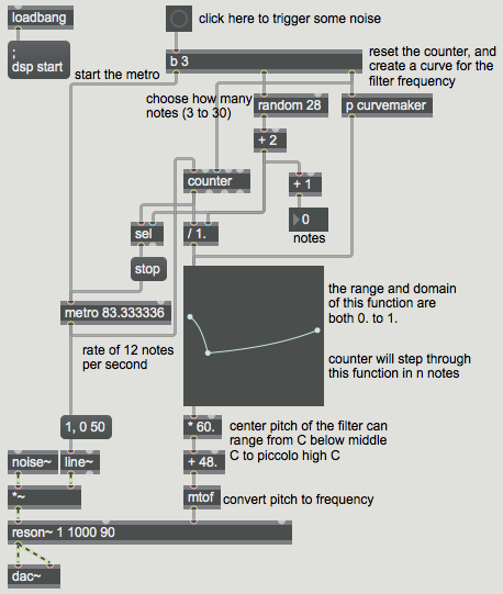
I believe that we respond to and recognize something about the shape of the change in a sound, and that shape forms a metaphorical sonic "gesture" in our minds. The "shape of the change" means the way in which some aspect of the sound (it could be any measurable parameter) or the music (it could be any characteristic we care about) changes over time: how radically it changes, and with what acceleration of change. That can be simply stated as the value of the parameter in question, depicted as a function of time. That is, the "gesture" can be depicted as a curve of change over time. Max's function object is a likely prospect for depicting that curve.
Based on that premise, this patch a) draws a curve by means of a simple process of randomly choosing three points and the curves between those points, b) randomly chooses a number of notes to play, and c) steps through that curve in that number of notes, using the curve as the center pitch of a resonant bandpass filter applied to short noise bursts. The number of notes is 3 to 30, note rate is a constant 12 per second, the amplitude of the white noise is constant, and the curve (described as taking place between 0 and 1 within the function object) is always somewhere within the range from MIDI 48 (C below middle C) to 108 (piano high C). Thus, the only variable factors are the duration of the gesture (number of notes) and the curve of the filter's change in pitch space.
The fact that this sounds "gestural", more so than linear change, implies that a) curves sound more physical than straight lines, and b) this very simple type of curve (three points with curves between them) is sufficiently interesting to sound gestural.
Example 13: Linear frequency vs. linear pitch
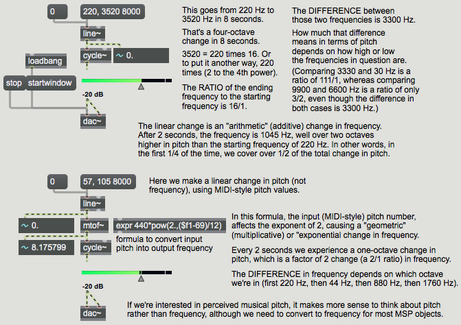
As expressed in Fechner's law, our subjective sensation of a phenomenon is often proportional to the logarithm of the empirical measurements of the intensity of the physical event that evokes that sensation. One example of that in musical contexts is that our sensation of changes in musical pitch are proportional to the logarithm of the change in the measured fundamental frequency of a tone. A linear arithmetic (additive) increase in successive frequencies, such as 100 Hz, 200 Hz, 300 hz, 400 Hz, 500 Hz, etc., would give us an impression of decreasing size of musical pitch intervals between those tones, in this case an octave followed by a perfect fifth followed by a perfect fourth followed by a major third, etc. You can think about this phenomenon in the opposite way, too: In order to give a linear impression of increase in pitch, you would need an exponentially increasing series of frequencies. For example, to give the effect of a linear chromatic ascent of equal-tempered semitones in a melody, the fundmental frequency of the successive tones would have to increase by a factor of the twelfth root of two for each interval.
This patch demonstrates that law. In the top part of the patch, a linear change in frequency is heard, covering a span of 3300 Hz, from 220 Hz to 3520 Hz, in 8 seconds. In the bottom part of the patch, a linear change in pitch is heard (converted to frequency before being sent to the cycle~ object) over the same range of frequency in the same total amount of time. In the former case, we hear a linear change in frequency as a logarithmic change in perceived pitch; the perceived pitch changes more quickly at first, and more slowly later. In the latter case, to get a sense of constant linear change in pitch, we need to use an exponential change in frequency, changing more slowly at first and more rapidly later. Listen to the two glissandi to see if you hear the difference.
Example 14: Plot an exponential curve
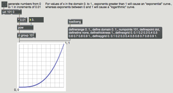
This patch allows you to see the effect of different exponents in a function that maps input values to output values with a power function. Input values between 0 and 1, taken to some power, will always yield output values from 0 to 1, provided that the exponent is greater than 0. (When the exponent is 0, the output values will all be 1. When the exponent is less than 0, the output values will be in the range from infinity to 1.) So, for exponential mapping of some range of input values to a corresponding range of output values, you can normalize the input values to the range 0 to 1, then take that to some power, then map the 0-to-1 results into the desired output range with a multiplication (scaling the size of the range) and an addition (to offset the range up or down). Note that exponents greater than 1 cause an exponential increase, whereas exponents between 0 and 1 cause a logarithmic increase.
Example 15: MSP transport demo
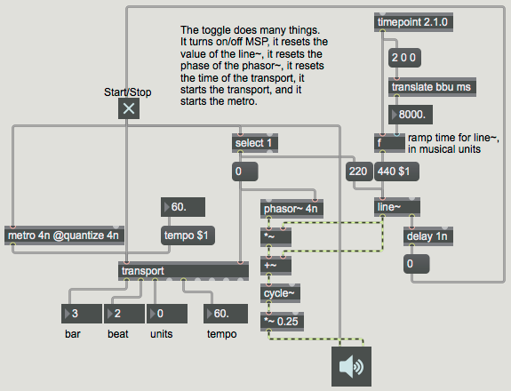
This patch demonstrates several capabilities, features, and techniques of the transport object for managing tempo-relative time, the translate object for converting between tempo-relative time and absolute time values, and the timing objects that can use tempo-relative timing such as metro, delay, timepoint, phasor~, and line~.
The transport object allows you to control timing in Max with a timeline-based model using musical time units such as bars and beats, a governing tempo (beat rate), and note values such as eighth notes, triplet sixteenth notes, etc.
In this example we use transport to start and stop musical time, schedule an event to happen at a particular moment in musical time, govern the timing of objects such as metro and delay that would usually use time specified in milliseconds, and control MSP objects such as phasor~ and line~ that would otherwise use a rate specified in Hertz or time in milliseconds.
This patch plays upward frequency glissandi, each one lasting for one beat, according to whatever tempo is set for the transport. For the first measure of musical time, it plays glissandi from 220 Hz to 440 Hz. Then, starting at the downbeat of measure 2, a timepoint object triggers a line~ object to move the overall range of the glissandi steadily upward so that two measures later, by the downbeat of measure 4, the glissandi are going from 440 Hz to 880 Hz. At the downbeat of measure 5, the program stops the transport and turns off MSP.
The timing interval of the metro is set to '4n', which will be exactly one quarter note at whatever tempo is specified. It is also quantized to the nearest quarter note on the timeline, with the '@quantize 4n' argument, so that it only sends out its bangs right on the beat according to the transport. The only thing the metro actually does in this patch is bang the transport object, which causes it to report information about its current state (location in time, tempo, etc.).
The MSP objects phasor~ and line~ are capable of understanding tempo-relative note values. You can also use the translate object to convert between absolute time values and musical time values if you need to. In this patch, it's not strictly necessary to convert the musical time interval '2 0 0' from bbu (bars, beats, and units) into ms (milliseconds), but we do so anyway to show that, no matter what the tempo we set for the transport, the translate object will make the proper conversion for us.
When expressing time in bbu format, it's important to understand the distinction between a position in time (a specific location on the transport's timeline, in terms of bars, beats, and ticks) and an interval of time (an amount of time). In the timepoint object, we're specifying a precise moment in time, bar 2 beat 1 exactly, whereas for the line~ object we're specifying an amount of time, 2 measures exactly, for it to reach its destination. In conversation we might use similar expressions to say these two things: "bar two" or "two bars"; but it's important to keep in mind that they're different things, and are expressed differently in bbu units. Also, notice that bbu units can be expressed in either of two ways, either as a space-separated list of three integers or as a dot-separated set of three integers.
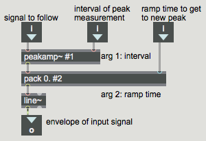
Example 16: Simple envelope follower
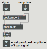
An "envelope follower" provides a smoothed global representation of the extreme amplitudes of a signal. It can be as rough or as detailed as you want it to be, depending on how much of the original signal you disregard in the evaluation of the peaks. Because sound signals tend to vary in both positive and negative directions around a central 0 value, it's best to evaluate the absolute values of the samples, so that peaks in the negative direction are easily compared to peaks in the positive direction. And because we care about the peaks, and not all the values that cross rapidly between positive peaks and negative peaks, it makes sense to disregard the non-peak values, and interpolate from one peak value to another.
One pretty simple way to obtain an amplitude envelope in real time is to periodically evaluate a short segment of the incoming signal -- usually 5 to 20 milliseconds at a time -- to determine the peak amplitude within that segment, then go to that peak value quickly (with sample-to-sample interpolation) from the previously detected peak value. The peakamp~ object provides a periodic report of the peak absolute value within a segment of a signal. This patch uses the line~ object to interpolate toward the peak value detected by peakamp~ during the time while peakamp~ is evaluating the next segment of the incoming signal. For many situations, this simple solution is good enough.
Note that realtime envelope following always requires some degree of latency (lag time) between the input signal and the amplitude envelope representation of that signal. It requires that each peak be determined, and the smoothing process to get from peak to peak, which is essentially a lowpass filtering process applied to the detected peaks, requires some small amount of time. In this patch, the peakamp~ interval takes some number of milliseconds -- during which the peak could occur at any time from the beginning to the end of that segment -- and the interpolation to that value takes the same number of milliseconds. Thus, the latency may be anywhere from n to 2n milliseconds. Still, for a value of n=10, for example, the lag will be only 10-20 ms, which is usually not a problematic amount of latency in a music performance.
Example 17: A variation on the simple envelope follower
This patch is very similar to the simple envelope follower, with the difference that in this patch the line~ object's time of interpolation to get to a detected peak value can be different from the peakamp~ object's interval of evaluation. If, for example, the peakamp~ interval is 10 ms and the line~ ramp time is 2.5 ms, the envelope follower latency will range from only 2.5 to 12.5 ms.
Example 18: Envelope follower with minimal latency
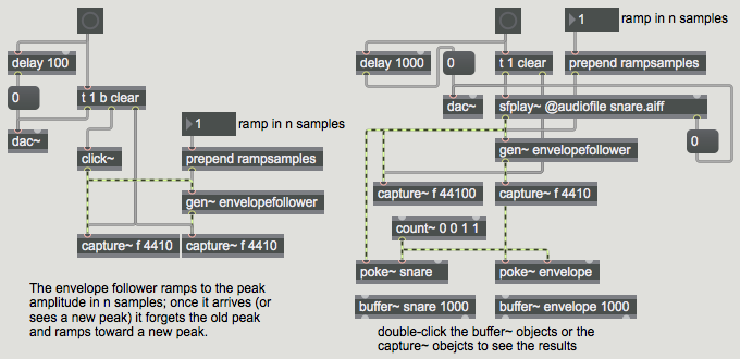
Audio signals change drastically and quickly. A 100 Hz sine tone goes from (absolute value) peak to peak in 5 milliseconds. An attempt to detect its peak amplitude in a lesser time interval might incorrectly evaluate a non-peak values as a peak. What we really care about is the shape of the peaks over time, so a certain amount of latency is necessary to represent that shape properly. And, if we plan to use the envelope to shape other sounds, some smoothing of the envelope is necessary to minimize the audio-rate modulation it causes when applied to other signals.
This patch demonstrates a realtime envelope follower that responds to the input signal with minimal latency. It responds to new peaks instantaneously (with sample-level immediacy), and smooths the envelope over any number of samples you specify. Because MSP works with audio one signal vector at a time, we can only get sample-level precision within a single MSP object. The gen~ object opens up that internal MSP world and allows you to program at the sample-level with MSP-like patching, even though it receives and sends its input and output vector by vector in MSP. (You can do the same in Java with the mxj~ object, or you can write your own MSP external object in C. But gen~ gives you sample-level programming capability in a MSP-like patching language. If need be, the code you create in gen~ can then be exported to be used in different formats, such as VST.)
Inside the gen~ object, the gen patch compares each incoming sample to the previously-detected peak value. If it detects a new peak, it begins to interpolate toward that new value over the course of the next n samples. That is, it calculates 1/n of the way from its previous output to the new peak, and outputs that value. As long as no new peak is detected, it will continue to interpolate to that new peak over n samples. Once it arrives at that peak (if it doesn't detect some new peak before it gets there), it resets itself and begins interpolating toward the next (presumably lesser) peak value. It's revising its opinion of the "peak" value every sample, so it will always be approaching the greatest value detected since the previous peak was reached.
The algorithm is described as well as possible inside the gen~ object, and the gen code is thoroughly commented. You can see its effect by looking inside the capture~ and buffer~ objects in the demo patch. If you want to use this code in a patch of your own, you can copy and paste the gen~ object or you can download the .gendsp file. Try different numbers for the 'rampsamples' parameter to get the enveloping effect you want.
Example 19: Saving and recalling presets in pattrstorage
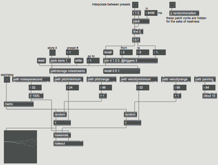
This patch demonstrates the use of pattr objects to store several attributes of a note-generating algorithm, and pattrstorage to store and recall preset values for all of those pattrs. In order to use the presets already designed for this patch, you will first need to download the file called notestreams.json and place it somewhere in the Max file search path.
A pattr object (the name stands for "patcher attribute") is a storage location for any Max message. A pattrstorage object stores the values of all the pattr objects in its patch at any given moment. Thus, you can think of pattrstorage as storing "snapshots" of the messages contained in all the pattr objects. Since pattrstorage can store many such snapshots and recall them later, you can set up any number of preset states for a patch to be in. When you recall one of those presets from pattrstorage, the pattr objects send out those stored values. In this way, you can instantly set any number of values in a patch just by specifying a single preset to pattrstorage. (For examples demonstrating the entire family of pattr-related objects in more detail, see examples 57-63 from a previous class.
Significantly, pattrstorage can also interpolate between presets, doing all of the necessary calculations for you, to obtain intermediate states between any two presets of pattr values. To get that interpolation effect, send pattrstorage a message that starts with the word 'recall', followed by one preset number (think of it as preset A) and then another preset number (think of that as preset B) and then a value from 0. to 1. specifying the desired location between preset A and preset B. So, if you wanted to get a smooth interpolation from one preset to another, you would send a series of messages that say recall [previouspreset] [nextpreset] [interpolationvalue], with each message having a different interpolation value progressing from 0 to 1.
The note-generating algorithm shown here produces MIDI notes at a specified rate (notes per second), with each note's pitch and velocity chosen randomly from within a constrained range of possibilities. Those ranges are specified by a minimum value (the lowest allowable random choice) and a range size (from minimum to maximum). For good measure, this patch also specifies a MIDI panning value to place the notes in the stereo field. Each of those paramenters is stored in a pattr: notespersecond, pitchminimum, pitchrange, velocityminimum, velocityrange, and panning. For this example, six presets of pattr values have been stored in the notestreams.json file, so you can recall any of those presets by specifying a number 1 to 6 in the number box labeled "go to".
To interpolate gradually from one preset to another, a portion of the patch allows you to choose a starting preset, an ending preset, and an interpolation time, and then when you click on the button labeled "interpolate between presets", it will construct a series of 'recall' messages to cause the desired transition from one preset to another. To spare you the tedium of doing that by hand, there's also a subpatch called randomtransition that will randomly choose a new preset to which to transition, and will choose a random amount of time from 1 to 10 seconds to get there. Try clicking on the button in the top right corner of the patch to hear some interpolations from one preset to another. The pitches are played by the noteout object, and are displayed by the multislider (set in "Reverse Point Scroll" slider style with a single slider).
Example 20: Turning a signal on or off
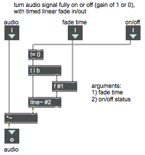
To turn an audio signal on or off instantly, Max provides the gate~ object. However, if you use gate~ to switch a signal on or off while MSP is on, you're likely to cause an unwanted click due to the sudden discontinuity in signal amplitude. To avoid such a click, you need to fade the sound in and out quickly by interpolating at signal rate between zero amplitude and full amplitude. MSP Tutorial 2 demonstrates the use of the line~ object and the *~ to fade from one amplitude to another instead of making an instantaneous switch.
This example provides a useful abstraction (subpatch) to turn a signal on or off by means of a linear fade-in or fade-out over a certain number of milliseconds. You can use this as an object in place of gate~, to avoid clicks when turning a signal on or off. Just download the patch and save it with the name onoff~. The fade time and the initial on/off setting of the object can be typed in as arguments when you create the object, and they will replace the #1 and #2 arguments in this subpatch. If you don't type in the second argument, the object will be off by default (the amplitude of the output will be 0). You should always type in a first argument for the fade time, otherwise the fade time would be 0 and the object would be no improvement over gate~.
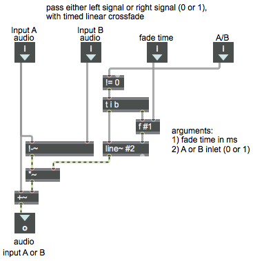
Example 21: Routing a signal to one of two destinations
This patch is quite similar to the onoff~ abstraction for turning a signal on or off with a fade-in or fade-out. Instead of just turning the signal on or off, though, this abstraction routes a signal to one of two outlets (with a fade from one to the other), which you can think of as destination A or destination B, based on whether the number in the right inlet is zero or non-zero.
You can use this as an object in place of gate~ 2, to avoid clicks when routing a signal out one or the other of two outlets. Just download the patch and save it with the name abgate~. The fade time and the initial A/B setting of the object can be typed in as arguments when you create the object, and they will replace the #1 and #2 arguments in this subpatch. If you don't type in the second argument, the object will route the incoming signal to the left outlet by default (the amplitude of the right outlet will be 0). You should always type in a first argument for the fade time, otherwise the fade time would be 0 and the object would cause a click whenever you switch between outlets.
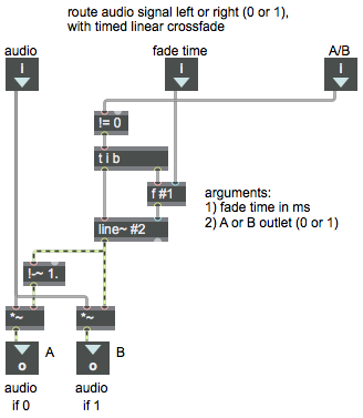
Example 22: Choosing between one of two signals
This patch is similar to the abgate~ abstraction for routing a signal to one of two outlets with a fade from one to the other. However, instead of routing one input signal to one of two outlets, this abstraction permits you to choose one of two input signals to send out its lone outlet.
You can use this as an object in place of selector~ 2, to avoid clicks when selecting between one or the other of two input signals. Just download the patch and save it with the name abswitch~. The fade time and the initial A/B setting of the object can be typed in as arguments when you create the object, and they will replace the #1 and #2 arguments in this subpatch. If you don't type in the second argument, the object will output the signal that's coming in the left inlet by default. You should always type in a first argument for the fade time, otherwise the fade time would be 0 and the object would cause a click whenever you switch between inlets.
Example 23: Turn an audio effect on or off
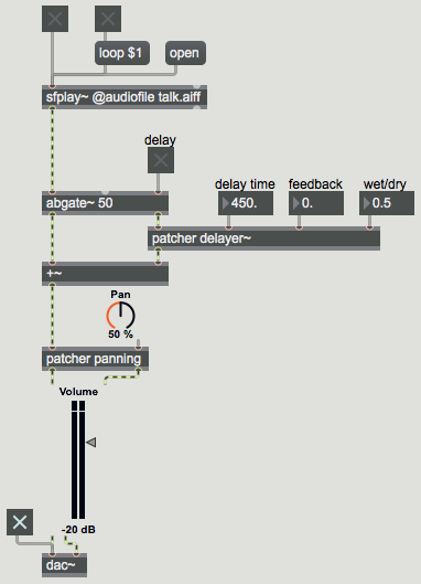
This patch shows a way to use the the abgate~ abstraction to route a signal through an audio effect processor, equivalent to using an effect insert in a mixer or a DAW. In order for this example to work correctly, you'll need to have that abstraction, saved with the name abgate~, in the Max file search path.
By default, abgate~ routes its input signal out its left outlet. So in this patch, the signal from sfplay~ is passed directly through abgate~ to the +~ object (and a 0 amplitude signal is passed out the right outlet of abgate~). When you want to insert the delay effect, you simply send a '1' in the right inlet of abgate~, and the incoming signal will be routed out its right outlet to the patcher delayer~. The contents of the patcher delayer~ shows a simple but effective example of how to implement delay with feedback. Like most good insert effects, this one includes the ability to control the "wet/dry" mix of the effect, so that you can still hear some of the original ("dry") input signal along with the effect. (Note, however, that this delay subpatch doesn't provide any protection against clicks if you change one of its parameters while sound is going through it.)
Example 24: Detect when an audio event occurs
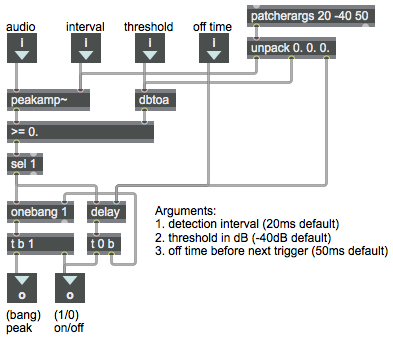
To detect when an audio event (such as a musical note) occurs, one straightforward method is to test whether the peak amplitude of the audio signal surpasses an established threshold that's slightly above the level of the ambient noise floor. The peakamp~ object periodically reports the greatest absolute value of amplitude that has occurred during the specified time interval. For quick response, that interval should usually be every 10 to 30 milliseconds. With a > (or >=) object, you can test whether that amplitude has surpassed the threshold you established. If so, the test will result in a "true" report of 1. Then you should ignore all subsequent 1 values until you get a 0 value indicating that the signal has dropped below the threshold. You can ignore the repeated 1 values with a change object, or, as in this example, convert the 1 into a 'bang' with sel 1 and then suppress the repeated bangs with the onebang object.
Some sounds may fluctuate significantly in amplitude within a note or phrase, such as a flute note with periodic tremolo. If those fluctuations cross the threshold, it could result in false reports of a new event. In order to avoid incorrectly interpreting such fluctuations as a new event, this patch provides an additional wait time after the signal dips below the threshold before it once again allows the report of a new event. In this patch, as long as the signal is above the threshold, and the "off time" is equal to or greater than the reporting interval, the delay object will be continually retriggered and won't send out the off (0) message. Only when the signal stays below the threshold for a time greater than the "off time" will the delay object send out its delayed bang to report the event has ended.
The three important parameters in this patch -- the testing interval, the amplitude threshold, and the off time -- can be specified as arguments to this object in the parent patch. If no arguments are provided, the patcherargs object provides default values for those parameters.
This page was last modified March 8, 2016.
Christopher Dobrian, dobrian@uci.edu