Example 1: Open a sound file and play it.
This page contains links to explanations and example Max patches that are intended to give instruction on some basic concepts of interactive arts programming using Max.
The examples were written for use by students in the Interactive Arts Programming course at UCI, and are made available on the WWW for all interested Max/MSP/Jitter users and instructors. If you use the text or examples provided here, please give due credit to the author, Christopher Dobrian.
There are also some examples from the previous years' classes available on the Web: MSP examples and Jitter examples from 2004's class, and some other examples from 2005's class, examples from 2006's class, examples from 2007's class, and examples from 2009's class.
While not specifically intended to teach Max programming, each chapter of Christopher Dobrian's algorithmic composition blog contains a Max program demonstrating the chapter's topic, many of which address fundamental concepts in programming algorithmic music and media composition.
You can find even more MSP examples on the professor's 2007 web page for Music 147: Computer Audio and Music Programming.
And you can find still more Max/MSP/Jitter examples from the Summer 2005 COSMOS course on "Computer Music and Computer Graphics".
Please note that all the examples from the years prior to 2009 are designed for versions of Max prior to Max 5. Therefore, when opened in Max 5 they may not appear quite as they were originally designed (and as they are depicted), and they may employ some techniques that seem antiquated or obsolete due to new features introduced in Max 5. However, they should all still work correctly.
[Each image below is linked to a file of JSON code containing the actual Max patch.
Right-click on an image to download the .maxpat file directly to disk, which you can then open in Max.]
Examples will be added after each class session.
March 30, 2010
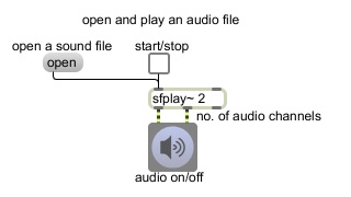
Example 1: Open a sound file and play it.
This shows an extremely bare-bones program for audio file playback.
1. Click on the speaker button (ezdac~ object) to turn audio on.
2. Click on the word "open" (message object) to open a dialog box that allows you to select a sound file. (In the dialog, select a WAVE or AIFF file and click Open.)
3. Click on the toggle object to start and stop playing. (The toggle alternately sends a "1" or "0" to the sfplay~ object, which sfplay~ interprets as "start" and "stop".)
The sfplay~ box is an MSP object. It performs an audio task: it plays sound files from disk and sends the audio signal out its outlets. The number 2 after sfplay~ is an 'argument', giving the object some additional information: that it should play in stereo, and thus should have two audio signal outlets. (The third outlet will send a notifying message when the soundfile is done playing, but this program doesn't use that outlet.) The speaker button (a.k.a. the ezdac~ object) is a 'user interface object'. It allows the user to interact with the program (in this case, by clicking on it with a mouse) and it performs a task (to turn audio on and off, and to play whatever audio signals it receives in its inlets as long as audio is turned on). Notice that the patch cords between the outlets of sfplay~ and ezdac~ are yellow and striped; that indicates that what is being passed between those objects is audio signal. The open object is a 'message box'. It's a user interface object, too. When clicked upon, it sends the message it contains (in this case, the word 'open') out the outlet to some other object. This is a message that sfplay~ understands. (If it were not, sfplay~ would print an error message in the Max window when it received an unfamiliar message.) The plain black patch cord indicates that what is passed between these objects is a single message that happens at a specific instant in time rather than an ongoing stream of audio data. The words 'start/stop' and 'audio on/off' are called comments. They don't do anything. They're just labels to give some information.
Here are a few thoughts for you to investigate on your own.
If you wanted audio to be turned on automatically when the patch is opened, and/or the 'Open File' dialog box to be opened automatically, how would you make that happen? (Hint: See loadbang.)
If you want to cause something to happen when the file is done playing, how would you do that? (Hint: Read about the right outlet of sfplay~.)
If you wanted to play the file at a different speed than the original, how would you do that? (Hint: Read about the right inlet of sfplay~.)
A single sfplay~ object can only play one sound file at a time, but it can actually access a choice of several preloaded sound files. How can you make it do that? (Hint: Read about the preload message to sfplay~.)
Suppose you'd like to be able just to pause sfplay~ and then have it resume playing from the spot where it left off rather than start from the beginning of the sound file again. Is that possible? (Hint: Read about the pause and resume messages to splay~.)
What if you want to start playback from the computer keyboard instead of with the mouse? (Hint: See key -- and/or keyup -- and select.)
Suppose you want to have control over the loudness of the file playback. What mathematical operation corresponds to amplification (gain control)? (Hint: See *~. See also gain~.)
April 1, 2010
Example 2: Control the volume and rate of a sound file.
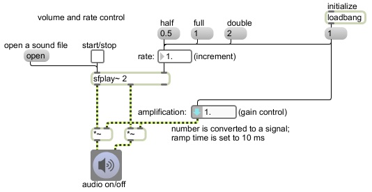
The right inlet of sfplay~ accepts a rate factor (increment factor) to control the speed of sound file playback. The factor can be supplied as a floating point number or as a MSP signal.
To control the amplitude of a signal, you need to multiply it by a gain factor -- greater than 1 to increase it, and between 0 and 1 to decrease it. The MSP object for multiplication is *~. Although *~ accepts either a float or a signal in its right inlet, it's usually best to control amplitude with a signal that doesn't change instantaneously, in order to avoid clicks in the sound. The number~ object used in this example actually has built-in linear interpolation that it uses when it receives a new number. When you change the value in the number~ object, it moves its output signal to that new value gradually over a certain amount of time, which you can set using the "Ramp Time in Milliseconds" attribute in the object's inspector. (The line~ object is also useful for moving from one value to another over a specified period of time, interpolating linearly sample-by-sample.)
Example 3: Demonstration of how message ordering works in Max.
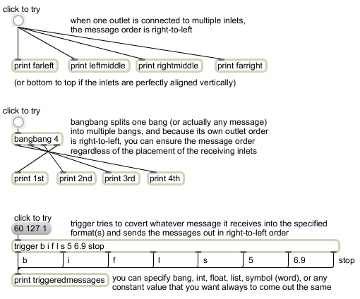
Even though Max is graphical, object-based, and event-driven (responds to user events like mouse clicks, key strokes, MIDI data, etc.), it's still sequential. Every message is sent (or scheduled to be sent) at a specific time, and nothing happens truly simultaneously. Therefore, it's important to be conscious of the precise order in which things occur. Study the example above to be sure you understand the way that Max orders messages.
Example 4: Timed counting in Max.
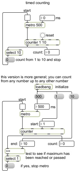
The upper example shows how to count from 1 to 10 at a specific rate (e.g., one count every 500 ms) and stop when you reach 10. The metro object sends out a bang message when it is turned on (when it receives a nonzero number in its left inlet), and continues to send out bang every x milliseconds (specified by the typed-in argument or by a number received in its right inlet). You can type in minimum and maximum values as arguments in the counter object. Every time it receives a bang, counter sends out its current count value and increments its internal counter to be ready to send out the next number. The select object looks for a particular number or word -- the integer 10 in this case -- and sends out a bang when it recognizes that message. That triggers a 0 to turn off the toggle which in turn turns off the metro.
The lower example is a more generalized version of the upper example. It allows you to specify any starting and ending value for the count. To avoid any problems that might occur if the ending value were to get set lower than the current count (in which case the counting might continue upward indefinitely), we use a greater-than-or-equal-to test, >=. If the number received in the left inlet is greater than or equal to the number specified in the right inlet, >= sends out a 1 ("true") message. That 1 will be detected by the select object, which will turn off the metro. Notice that loadbang is used in this example to initialize the settings of all the user interface objects (number boxes) and send those values into the necessary inlets of other objects.
If you just can't get enough of this (banal but fundamental) topic of "counting", you can read more on my Algorithmic Composition blog, specifically in the chapters titled "Timed counting" and "Counting through a List".
April 6, 2010
Example 5: Read MIDI pitches from a lookup table.
To store any series of integer numbers as an array, the table object is most convenient. You can look up the stored numbers by referring to their index location within the table. Thus, you can read through the numbers in the array, in order, using a counter object.
The makenote object allows you to easily attach a velocity and a duration to a pitch number. It keeps track of the pitches it has received, and the desired duration of each note, and sends out the same pitch with a velocity of 0 after the specified time interval.
For a smooth, linearly-changing sense of tempo, it's better to refer to the rate of events rather than the time interval in milliseconds. (Why is that?) So this patch lets you set and/or modify the note rate, and then converts that into milliseconds for the metro object. Note that it also sends the time interval to the right inlet of makenote so that the note durations are appropriate for the tempo at which the notes are being generated.
April 8, 2010
Example 6: Play a QuickTime movie with Jitter.
The jit.qt.movie object can open (read) a .mov file (or really any media file that QuickTime is capable of dealing with) and start playing it, loading its visual content into its internal Jitter matrix. But that matrix is only made visible when you send it a bang message, which causes it to send out a jit_matrix message to jit.window telling it where in memory to look to get the data to be displayed. Thus, the 'playing' of the movie (loading it in from the disk) and the displaying of it in jit.window are really two separate operations.
April 13, 2010
Example 7: Random number generators: random and urn.
This patch demonstrates the two simplest objects for generating random numbers. Every time it receives a bang in its left inlet, the random object generates a random integer in the range from 0 to one less than its argument. (For example, if you tell it to generate one of 12 random numbers, it will choose a number from 0 through 11 inclusive.) Note that this includes the possibility that successive random choices may appear to generate what seem to be patterns, especially if it's choosing from among a small range of possibilities. That's because repetition is possible. The urn object functions in much the same way, but it always generates a unique number (i.e., it doesn't repeat a number). Once it has no more unique numbers available within the specified range, it sends a bang out its right outlet indicating "I'm all out of possibilities" instead of sending a number out its left outlet. The clear message resets urn. Can you figure out how to make urn reset itself and try again when it's out of numbers to choose?
In this example, the random numbers are used as pitch information, generating an arbitrary atonal melody. That's certainly not the most interesting thing to do with random numbers, but it does demonstrate what arbitrary atonal melody sounds like, and 'sonifies' randomness pretty successfully.
There are several other objects for generating random numbers.
My algorithmic composition blog has several chapters on randomness, beginning with (intuitively enough) the chapter titled "Randomness".
Example 8: Random video editing.
This is a program for random editing of a video by periodically leaping to randomly-chosen times in the video and playing from there. The jit.qt.movie object here has its attributes initialized such that: a) it will adapt the dimensions of its matrix based on the dimensions of the movie that is read in, b) it will not automatically start, c) it will not loop, and d) it will only send out new frames of video without repeating a frame. When a movie is read in, a read message comes out the right outlet of jit.qt.movie; if the read was successful (the flag at the end of the read message is 1) it will trigger queries for attributes of the movie, namely its time units, duration, frames per second, and dimensions. The results of those queries are used to set the size of the display window (using moviedim), the rate of the frame-displaying metronome (using fps), and the range to use for the random time choices (using duration and timescale). The random range is set as follows: the timescale of the movie (QuickTime time units per second) is multiplied by the interval between edits (in seconds) and subtracted from the total duration. That ensures that each random edit will start at a time in in the movie that will allow the edit to play without hitting the end of the movie. When the toggle is turned on the random location choosing metro is turned on to choose the first edit location, the movie is started, and the display qmetro is started. A new randomly-chosen time message will be sent to the jit.qt.movie object at the specified rate.
Example 9: Linear mapping of one range to another.
This program shows the formula for linear mapping of one range to another, and implements the formula using basic Max math objects. One can use the objects zmap and scale to do this task more simply, but this example demonstrates the formula explicitly.
Example 10: Exponential mapping.
A linear fade-in or fade-out of audio is okay for quick changes that take place in a fraction of a second, but for slower fades one should generally take into account that our subjective sense of loudness more closely conforms to an exponential change in amplitude. This patch allows you to use the slider (or the mod wheel from a MIDI controller) to control the amplitude of white noise in one of three different ways: with straight linear mapping, exponentially (with an exponent of 4), or using a range of 60 decibels. A linear fade subjectively seems to have too drastic an effect with low slider positions, and too slight an effect at higher slider positions. The exponential curve is closer to our sense of loudness, but at lower slider positions the amplitude is too low. The dbtoa object allows us to map the input to a desired range of decibels (0 to -60 is suitable for most listening environments) and then convert that to amplitude. The linear change in decibels produces an exponential change in amplitude that is similar to our perception of loudness, so a linear change in the input gives a pretty linear sense of change of loudness.
Example 11: Linear interpolation over time.
The line object sends out a periodic series of numbers that progress to some new value over a certain amount of time. The input to line is a destination value (where it should eventually arrive), a transition time (how long it should take to get there), and a time interval between oututs (how often it should send out intermediate values along the way). The left part of this patch shows the use of line to generate integers that are used as pitches. (The integers could just as well be used as indices in a table to look up a non-linear series of numbers.) The right part of the patch uses line to generate floats from 0 to 1 that are uses as a multiplier to control the brightness of an image in a Jitter matrix. The pack object takes in several numbers (three in this case) and sends them out together as a single list, which line interprets as destination value, transition time, and output interval. Each output of line first goes to the right inlet of the jit.op object (to be used as the multiplier) and then sends a bang to the jit.matrix object to send out its jit_matrix.
Example 12: Linear interpolation of audio.
For linear interpolation of a MSP signal, the line~ object sends out a signal that progress to some new value over a certain amount of time interpolating sample-by-sample along the way. The input to line~ is a pair of numbers representing a destination value (where it should eventually arrive) and a transition time (how long it should take to get there). It can receive multiple pairs of numbers in a single message, and it will use the pairs in order, starting each new pair when the previous transition has finished. The left part of this patch shows the use of line~ to generate a short (50ms) amplitude envelope for a burst of white noise. It also uses another line~ to pan the signal back and forth between audio channels 1 and 2, by turning up one channel while turning down the other channel. The right part of the patch uses line~ to quickly smooth out transitions caused by new Max messages coming from the slider. Instead of instantaneous changes when a new number comes from the slider (which might cause clicks in the audio signal), line~ interpolates over 20ms (882 samples).
Notice that, although this patch demonstrates the line~ object, the actual changes to the audio are usually not linear, for perceptual reasons. The slider (which was set in its Inspector to send out values from -61 to 0) is expressing decibels, which are converted to amplitude by the dbtoa object. then smoothed with a linear interpolation between successive values. The panning portion of the patch uses linear fades for the gain of the two channels, but actually applies the square root of those gain values to create a constant-power panning effect. The gain~ object (the volume control for the white noise) uses an exponential curve for gain change that is perceptually preferable to a straight linear scale.
April 15, 2010
Example 13: Live recording into RAM.
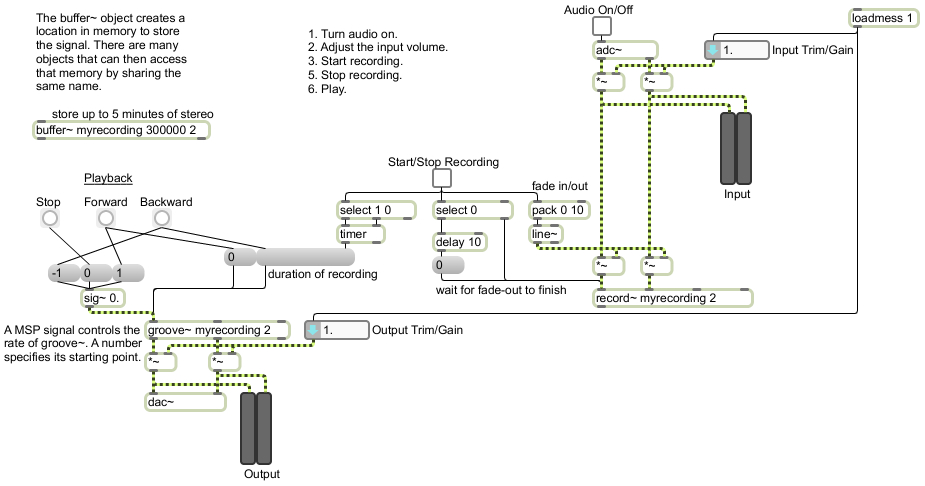
This shows how to record into a RAM buffer, and how to play back the contents of the buffer at any rate (even backward by using a negative rate) starting at any point in the buffer. A timer is used to keep track of the duration of the recording. The example also demonstrates how one might use a quick fade-in and fade-out to avoid clicks when doing realtime capture during a performance.
Example 14: Live recording into a sound file.
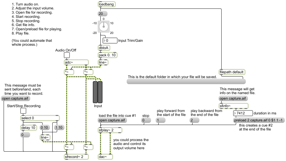
This shows how to record into a sound file, and how to play back the contents of the file. The example also demonstrates how you can use a quick fade-in and fade-out to avoid clicks when doing realtime capture during a performance. To play the file back in reverse, you have to create a rather complicated preload cue in which you specify the name of the file, the cue number, the start point and end point (put the point that occurs earlier in the file first, even though you intend to play backward from end point to start point), then the number 1 (that's a flag to tell sfplay~ that it should also preload some data at the end of the cue because you intend to play backward), and then the rate (-1 for backward at normal speed). So, for example, to make a cue #2 that will play starting 10 seconds into the file and reading backward to the beginning of the file, you would send the message preload 2 capture.aif 0 10000 1 -1.
April 20, 2010
Example 15: Using key presses and releases.
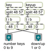
Using both the key and keyup objects, you can tell when a key was pressed and when it was released. The split object allows you to isolate a range of numbers; it passes only the specified range of numbers out its left outlet, and passes all other numbers out its right outlet. The numbered keys 0 to 9 correspond to ASCII codes 48 to 57, so it's easy to isolate those keys, and subtracting 48 brings those numbers down into the range 0 to 9. In this example, we trigger a 1 when the key is pressed and a 0 when it is released--in the manner of a MIDI key producing nonzero and zero velocities--and then pass on the 0-to-9 number. This seems like a potentially useful function for using the number keys as button presses (momentary toggles) to control your Max program. The outlet objects make this program useful as an object in some other patch. When used as an object in a parent patch, this program will first send the down/up status of the key out the right outlet, and it will then send the key number (0 to 9) out the left outlet.
Example 16: Using arrow keys to control a slider.
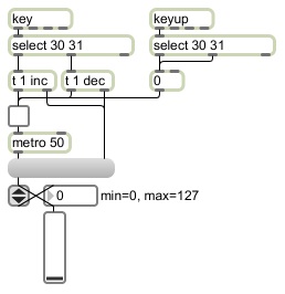
The up-down arrow keys seem like reasonable keys to use for incrementing or decrementing a number box or a slider. But rather than require a new key press for each step up or down, you can use a fast metro to trigger messages continuously as long as the key is pressed. There are several ways one could implement this in Max; here's one example.
There's an object called incdec that is designed to be interconnected with a number box in the way that's shown here. It keeps track of the value in the number box and takes inc and dec messages to increment or decrement the number box. The key object first triggers the correct message -- inc or dec -- to set the contents of the message box, and then it turns on a metro to repeatedly send that message. When the key is released, it triggers a 0 to stop the metro. The number box has been set in the Inspector to have a minimum value of 0 and a maximum value of 127, so attempts to decrement it or increment it beyond those bounds will be limited (clipped) to those values.
Example 17: Pass a certain percentage of bangs.
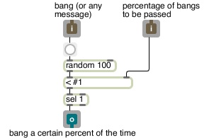
To make a random decision between two things, you can use the decide object. To make a probabilistic decision between two things, with one thing being more likely than the other, you can use the random object to choose randomly from a larger set of numbers, then assign a majority of those choices to mean one thing (and the remaining minority to mean the other thing). An easy way to do this is with the < object. In this example, a bang in the left inlet will choose a random number from 0 to 99, and that number will then be tested to see if it's less than some specified 'percentage' from 0 to 100. If it is, the < object will send out a 1, causing a bang to be sent out the outlet. This means that, over a fairly large number of incoming bang messages, approximately the specified percentage of them will result in output.
The percentage can be sent in the right inlet, or specified as a typed-in argument in the parent patch. The #1 argument in the < object means that when this patch is used as an object in another program the #1 will be replaced by whatever is typed in as an argument to the object in the parent patch. If there is no typed-in argument in the parent patch, the #1 defaults to 0.
Example 18: Repeated notes at 6 related tempi, with different probabilities.
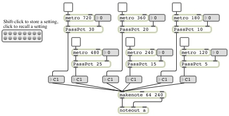
This example (taken from Tutorial 37 in the original Max tutorials) demonstrates one way the "passpct" program from the previous example could be used. This program has six metro objects set to six harmonically-related tempi. The bang messages from those metros are filtered probabilistically by the passpct objects, and will thus trigger note messages with the specified likelihoods.
A preset object stores "snapshots" of the state of the user interface objects in the patch (in this case, the toggles and number boxes). By clicking on the different preset buttons (or by sending the desired preset number to the preset object) one can recall a previously-stored snapshot. Try clicking on the preset buttons (in any order, ending with preset 16) to perform a simple interactive algorithmic composition.
April 22, 2010
Example 19: Bandpass filter swept with a LFO.
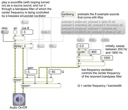
This example demonstrates one of MSP's many filter objects -- the resonant bandpass filter reson~ -- and demonstrates how a parameter of that filter -- in this case its center frequency -- can be easily modulated by a low-frequency control oscillator (cycle~). The range of cycle~ is between 1 and -1, but that range can be amplified by multiplication, and can be offset by addition. In this case, it is initially set to sweep plus and minus 800 Hz around an offset of 1000 Hz, so the range of the center frequency will be between 200 Hz and 1800 Hz. The rate of the LFO is initially set to 0.5 Hz, so it completes one sweep every 2 seconds.
The sfplay~ object is initialized to have eight preloaded cues, numbered 2 through 9, using the eight sound files that are supplied in the Max examples folder, and is set to loop on playback. The filter is intialized with a Q factor of 50 and a gain of 3 (because the high Q factor will tend to reduce the overall volume of the sound). Turn on audio, and click the "go" button. Try changing the various parameters, and listen to the effect on different sounds.
Example 20: A variable-mode filter: biquad~.
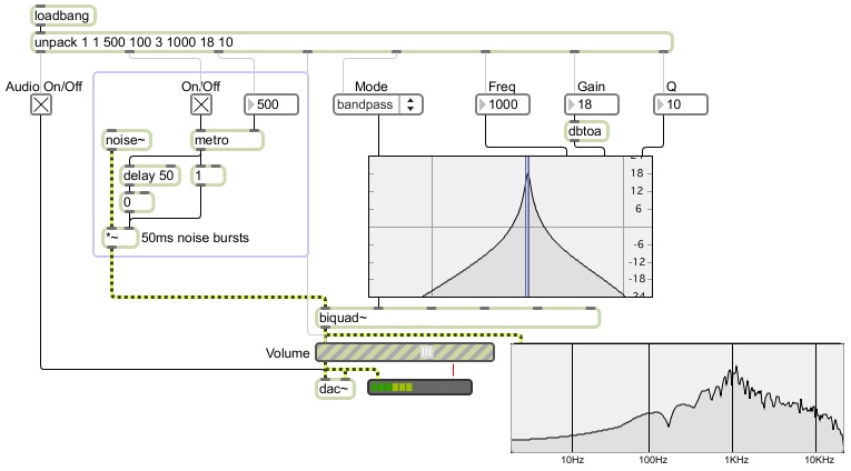
This patch allows you to try out various filter settings of the biquad~ object, via the filtergraph~ object. For adjusting the parameters, you can drag on filtergraph~ with the mouse, or you can send values in its three rightmost inlets for frequency, gain, and Q. The spectroscope~ object tries to draw the spectrum of the signal.
If you want to change the coefficients of biquad~ in real time while a sound is playing, it's usually better to use MSP signals rather than individual Max messages, to avoid causing clicks. (It doesn't really matter in this example, since the source signal is noise anyway.) The next example demonstrates two ways to do that.
Example 21: Smooth filter changes.
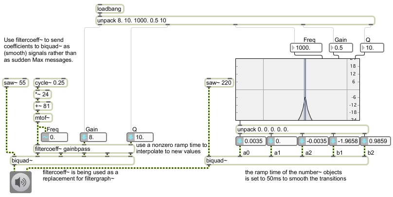
If you want to change the coefficients of biquad~ in real time while a sound is playing, it's usually better to use MSP signals rather than individual Max messages, to avoid causing clicks. In that case, you should replace filtergraph~ with filtercoeff~ and send the frequency, gain, and Q parameters into filtercoeff~ as smooth signals (as shown in the left portion of the example). Or, if you also need the graphic interface capabilities of filtergraph, use line~ -- or number~ with a nonzero ramp time -- as an intermediary between filtergraph~ and biquad~, to smooth the transitions with interpolation (as shown in the right portion of the example).
April 27, 2010
Example 22: Switching and mixing audio processes.
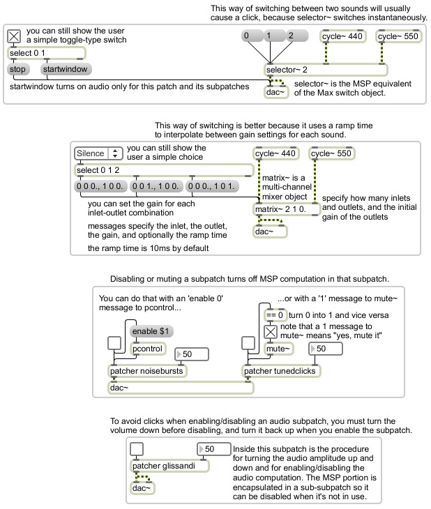
As you get more involved in programming audio, it's likely that you'll want to have multiple sound possibilities available in your program, that you can switch on and off as needed. You might want to take a look at MSP Tutorial 5: Turning signals On and Off to learn about some basic ways of doing that. However, that chapter leaves out the following pretty crucial issue. In most cases you want to make sure the volume of the sound is 0 when you turn it on or off, in order to avoid clicks. So any time you turn a sound on or off, or disable a part of your program (to save on needless computation), or switch from one sound to another, you usually will want to do a quick fade-in or fade-out rather than an instantaneous switch on or off. There are lots of strategies and techniques you might use for that. This patch that shows a couple of useful tricks.
The selector~ object is quick and handy, but usually is not appropriate for switching audio signals in real time. A quick cross-fade between the signals is what you really want. The matrix~ object, which serves as a multi-channel mixer, is very handy for that purpose. The pcontrol and mute~ objects provide two different ways of silencing and disabling audio in a subpatch. It's a good idea to disable subpatches that you're not listening to, in order to reduce needless computation in MSP, especially if you have a lot of audio processing going on. But you usually will want to fade the audio to 0 before disabling a subpatch. The bottom part of this example shows a way to do that, by encapsulating the fading and disabling in a subpatch, and encapsulating the actual audio processing in a sub-subpatch within that, which you can disable when it's not in use.
Example 23: Polyphony requires multiple objects.
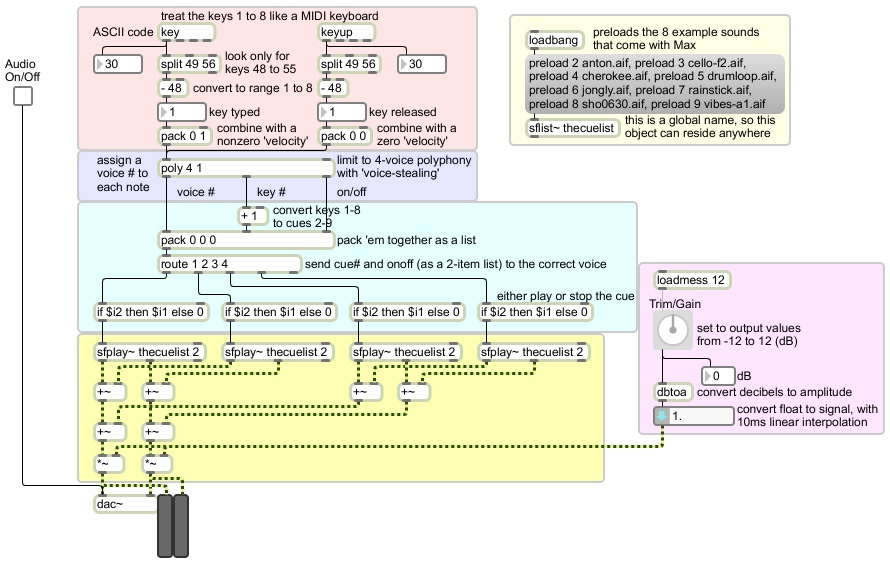
Any given MSP patch cord represents a single channel of audio. If you want to generate or process multiple sounds or channels, you need to treat each sound or channel separately. For example, each sfplay~ object can have multiple loaded sound cues so that it's ready to play any one of several files, but it can only play one sound file at any given instant. And if it's a stereo file you need to treat each channel separately for mixing, processing, etc. This patch demonstrates that. The patch has several components, outlined by different color regions.
The top (pink) part of the patch doesn't have anything to do with audio. It shows the use of key and keyup to detect key presses and releases, the use of split to isolate a particular range of ASCII values corresponding to the number keys 1 through 8, and then the use of pack objects to attach a 1 to each key press and a 0 to each key release, making each key into a unique momentary button press, analogous to a simple MIDI-like keyboard. This lets you use key presses to trigger the starting and stopping of sound files.
The next (blue) portion of the patch demonstrates the poly object, which supplies a unique voice number to each pitch and velocity pair it receives. The argument 4 determines how many voices poly will allow, and the argument 1 is a flag that turns on "voice stealing". When voice stealing is on, when poly has received more than its maximum number of notes (4 in this case) it sends out a note-off for its oldest note (a velocity of 0 and the pitch number) before it sends out the note-on for its newly-received note. It treats the lists it receives as if they were pitch-velocity pairs. This is a good way to limit the number of notes you generate at any given moment.
The next (green) section adds 1 to the key numbers (1 through 8) to convert them into cue numbers for sfplay~ (2 through 9), and packs the voice number, cue number, and 'velocity' (1 or 0) together as a list. The route object looks at incoming lists, and compares the first item in each incoming list (in this case, the voice number) to its own arguments. If it finds a match, it routes the rest of the list out the corresponding outlet. This is a good way to direct messages to a particular destination. Here it directs each cue to a unique sfplay~ object so that multiple cues can be played simultaneously. The if objects say, in effect, if the second number (the 'velocity') is nonzero, then send out the cue number (to play the cue), otherwise send out 0 (to stop the cue). [Geeky side-note: In this particular instance, you could replace the if objects with * objects. Do you see why? But the if object more explicitly explains what's going on.]
The next (yellow) section demonstrates the mixing of multiple sound generators. The sfplay~ objects play in stereo, so the +~ objects add all the left channels together and all the right channels together before passing them to the dac~. Once they have all been added (mixed) together, they go through *~ objects to give some control over the overall amplitude, because the four mixed sound files could potentially add up to a signal greater than 1 which would get clipped when sent to the dac~.
But how do the sfplay~ objects know what the cue numbers mean? They all have a common argument "thecuelist" that causes them to refer to a sflist~ object with the same argument. This is a good way to keep all cues localized in one place, to which multiple sfplay~ objects can refer. In the upper-right (orange) portion of the patch we have initially preloaded cue numbers 2 through 9 into a sflist~ object named "thecuelist". That cue information is shared by all sfplay~ objects with that same argument.
The lower-right (violet) portion of the patch gives the user a dial with which to control the output volume up to + or - 12 decibels. Those amplitude changes are smoothed with a number~ object that sends out the value as a signal, smoothed with a 10-millisecond ramp time whenever it receives a float in its inlet. Notice that the output signal is also being sent to meter~ objects, so you can monitor the effects of the volume control.
Example 24: Generating a simple 2-operator FM tone.
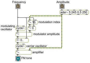
In order to enable and disable portions of an audio program easily, and to be able to reuse them multiple times, you will probably want to encapsulate an entire audio-generating or audio-processing procedure inside a single patch with inlets and outlets so that it can be used as a subpatch object in some other patch (as demonstrated in Example 22 above). This patch shows an example of a simple 2-oscillator frequency modulation tone generator that could easily be used as a subpatch in some other patch. (In Example 26 below, this patch is modified to make it fully functional as one voice of a polyphonic synthesizer.)
The patch has two inlets, for frequency and amplitude, which can receive either floats or MSP signals. The lower cycle~ object is the carrier oscillator (the one we actually will hear) and the upper cycle~ object is the modulating oscillator (the output of which will be used to modulate the frequency of the carrier oscillator.
The frequency value that comes in the left inlet is used to set the base frequency of the carrier oscillator (in the right inlet of the +~ object), the frequency of the modulating oscillator (in the left inlet of the upper cycle~ object) and as a factor in determining the depth (amplitude) of the modulation (in the right inlet of the *~ object). For a fuller explanation of frequency modulation synthesis, read MSP Tutorial 11: Frequency Modulation.The adsr~ object outputs a signal that follows the shape of an ADSR envelope, which is useful for shaping the amplitude of another signal, or for controlling a parameter of another object (such as the cutoff frequency of a lowpass filter). As is standard for ADSR envelopes, the attack time, decay time, sustain level, and release time describe the shape of the envelope. In this example, the envelope will rise to full amplitude in 5 milliseconds, decay over 245 milliseconds to a sustain level that is 0.5 as great as its peak (attack) level, and then when the note is released the envelope will fade out in 250 milliseconds. The overall amplitude of the envelope will be scaled by whatever value comes in adsr~'s left inlet (i.e., whatever comes in the right inlet object in this patch). When adsr~ receives a value of 0 in its left inlet, that triggers the release, sending the amplitude of the ADSR envelope to 0 in 250 milliseconds. A new nonzero value then retriggers the start of the envelope. Notice that the ADSR envelope is used to scale the amplitude of the output tone, and the same envelope is used (multiplied by a factor of 10) as the modulation index (modulation amplitude divided by modulation frequency). In this way, the tone will get brighter (have more, stronger upper partials) as it gets louder, and will become purer as it gets softer.
You can see that this patch expects to get both a frequency value and an amplitude value in its inlets. The amplitude value will trigger the ADSR envelope and scale its overall amplitude. The frequency value will set the parameters of the carrier and modulator oscillators. These two values could arrive together at the start of a note, perhaps derived from the key and velocity values of a MIDI note-on message.
The next example shows this patch being used as a subpatch in a larger patch. You will need to download this patch and save it with the name "FMtone~" in order for the next example to work.
Example 25: Polyphony with multiple copies of a MSP subpatch.
This example shows the patch from the previous example being used as a subpatch in a larger patch. You will need to download the patch from Example 24 and save it with the name "FMtone~" in order for this example to work.
Once you have made a subpatch that reliably generates or processes audio, you can use it as many times as you'd like in other patches. The method shown in this example -- using many copies of the same subpatch -- is not really the preferred way to achieve polyphony. Compare this example to Example 27 in which the preferred poly~ object is used to load multiple copies of the same audio subpatch. However, this example does explicitly show how command messages can be routed to multiple copies (voices) of a polyphonic synthesis process, and how those independent voices can be remixed as a single signal. That's effectively what must happen in any polyphonic synthesizer, and it's essentially the way that the poly~ object works internally, so it's worth understanding this example before looking at poly~.
In this example, the borax object generates and assigns a unique voice number for every MIDI note-on message that comes in, and assigns the same voice number to the corresponding note-off message. In this sense it's very similar to the poly object used in Example 23. (The borax object also provides other data about incoming note messages, which are not used in this example.) The pitch and velocity information from the MIDI note messages gets translated into frequency and amplitude information suitable for the FMtone~ subpatch, those numbers get packed as a list along with their corresponding voice number, and the voice number is then used to route that frequency and amplitude information to one of eight copies of the FMtone~ object. The sound from those FMtone~ objects is mixed together in the +~ objects, scaled by a factor of 1/8 to prevent the output signal from clipping, and sent to the dac~.
Example 26: A subpatch suitable for use in poly~.
This patch demonstrates how one might make an audio patch that can serve as a voice in a polyphonic synthesizer. It's quite similar to the FMtone~ patch shown in Example 24, but with some important modifications that make it suitable for use with the poly~ object so that it can be used polyphonically. Some important features been added in this example.
Notice, first of all, that in addition to the inlets and outlet, this patch has in objects and an out~ object. These objects are specifically needed in conjunction with the poly~ object. Wherever you would normally have inlets and outlets for using a patch as a subpatch, you should use the equivalent in and out objects for using the patch in poly~. These will then appear as inlets and outlets in the poly~ object that loads this patch as a subpatch. For inlets and outlets that will handle MSP signals, use the in~ and out~ objects instead. This patch uses both -- inlets and an outlet and ins and an out~ -- so the patch can be used either as a normal subpatch or inside a poly~.
The pack object in this patch allows the parent patch to send in the frequency and amplitude information either as separate numbers in the two inlets or as a single two-item list in the left inlet, similarly to the way that noteout and many other Max objects work. But regardless of how the information is sent in, when something comes in the left inlet pack will send out both items, and unpack will send them to the proper place.
The amplitude information is used by two different adsr~ objects, one for controlling the output amplitude and one for controlling the modulation index. The modulation envelope has a faster attack time and a slower decay time than the amplitude envelope, so the timbre evolves slightly differently from the amplitude. The legato 1 message to adsr~ tells it to turn "legato" playing on. That means that when adsr~ starts a new envelope it should start from whatever amplitude it is currently at, rather than leap to 0 to start the new envelope. This will give a smoother (more legato) transition from one note to another if a new note is triggered before the release time of the previous note has fully elapsed.
The FM portion of the synthesizer is encapsulated inside a patcher object (the p FM~ subpatch). This is done just for organization, to make the window a little less complex visually, not for any particular functional reason.
The thispoly~ object is important because it allows a subpatch inside poly~ to communicate some things about its state to the poly~ that contains it -- things that might be unique to that particular voice. The most significant things you can do with thispoly~ are to mute/unmute a voice, or to set/unset its "busy" status. You can stop computation in a particular voice of a poly~ by sending a mute 1 message to a thispoly~ object in the voice patch. To restart MSP computation in that voice, send mute 0 to thispoly~. An extremely useful feature of the adsr~ object is that when it completes an envelope it sends a mute 1 message out its third outlet, and when it starts a new envelope it sends out mute 0. This is specifically meant to be sent to thispoly~ by the adsr~ that is controlling amplitude, as is done in this example, in order to turn off computation in the voice whenever the amplitude is 0. For voice allocation in response to note or midinote messages, poly~ needs to know whether a voice is already busy synthesizing or whether it's available to synthesize a new note. If the signal in the inlet of thispoly~ is 0, poly~ considers that the voice is available to play a new note, but if the signal in the inlet of thispoly~ is nonzero poly~ knows that that voice is already busy. For this purpose, too, the adsr~ that controls the amplitude is the perfect object to provide the "busy" or "not busy" signal, because when the envelope is at 0 that means that the note is over and the voice is once again available. Thus, thispoly~ is a necessary object for eliminating unnecessary MSP computation and for voice allocation, and its logical partner is an adsr~ object that is controlling the patch's output amplitude.
The next example shows this patch being used inside a poly~ object. You will need to download this patch and save it with the name "FMsynth~" in order for the next example to work.
Example 27: Polyphony with the poly~ object.
This example shows the patch from the previous example being used as a subpatch inside the poly~ object. You will need to download the patch from Example 26 and save it with the name "FMsynth~" in order for this example to work.
The poly~ object is a way of managing multiple copies of the same subpatch, primarily as a way of achieving polyphony in MSP. To do polyphonic audio with poly~, you must first design a subpatch that either generates or processes MSP audio and sends it out, and you'll design it in such a way that it can respond to control input from a parent patch, and you'll include in, in~, out, and out~ objects (in place of, or in addition to, inlet and outlet objects) so that it will work inside poly, as demonstrated in Example 26.
This example demonstrates one common way to address the individual voices in a poly~: using the target message. Think of poly~ as containing multiple copies of the same patch, with the ability to control each of those copies independently. In this example, the poly~ contains eight instances of the FMsynth~ subpatch. As you know from the discussion of that patch, it can receive frequency and amplitude information as a list in its left inlet, and when it does, it will play a note with FM synthesis. To address each one of those eight copies individually, you need to precede the frequency and amplitude information with a target message that specifies which voice (which copy of the subpatch) will receive subsequent messages. For example, if poly~ receives the message target 1, it will then direct all subsequent messages to copy 1 of its subpatch.
Here we use the poly object (no tilde!) to ascribe a unique voice number to each incoming MIDI note-on message. However, the voice number comes out of the left outlet of the poly object after the velocity and pitch information, so if we want to use the voice number as part of the target message, we need to do some message reordering. The velocity comes out the right outlet of poly, gets turned into an appropriate amplitude by the expr object, and is held in the right inlet of the pack object. The pitch comes out the middle outlet of poly and gets held in the right inlet of the swap object. Finally, the assigned voice number comes out the left outlet of poly and goes to the left inlet of swap. (The function of the swap object is to swap the message order of its messages. What comes in the left inlet goes out the right outlet first, and then whatever had come in the right inlet is sent out the left outlet.) The voice number thus goes out the right outlet of swap and becomes part of the target message, telling poly~ which voice to address. Then the MIDI pitch number comes out the left outlet of swap, gets converted to frequency by the mtof object, gets packed together with the amplitude information in pack, and gets sent to the left inlet of poly~ which directs it to whichever voice is currently targeted. The same process applies for every MIDI note that comes in, but each note will be targeted at a different voice of the poly~ (because poly will have assigned and targeted a unique voice number from 1 to 8). Because it's conceivable that we might receive eight nearly simultaneous loud notes at the same time, we've chosen to scale the overall amplitude of the output of poly~ by a factor of 1/8.
Regardless of whether the control information is actually coming from MIDI input, and regardless of how the control information will be used inside the subpatch of poly~, the target message is the standard way to send any information into a specific voice of the poly~. It tells poly~ in advance which voice you wish to apply the information to, and all subsequent messages will be sent to that voice. If you wish to send the same message to all voices at once, precede the message with a target 0 message, which targets all voices.
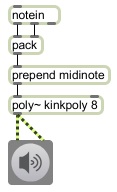
Example 28: Phase distortion synthesis in a poly~ subpatch.
This shows an implementation of phase distortion synthesis in MSP -- using the phasor~, kink~, and cycle~ objects -- in a patch that is designed to be used inside the poly~ object. For an explanation of this sort of phase distortion synthesis, see Example 30 below. The main point of this example, though, is to show how a synthesis patch can be designed to respond directly to MIDI input. Although the method of synthesis is different, the basic design of this patch is very similar to the FM synthesis poly~ module presented in Example 26 above. One noticeable difference is that instead of expecting frequency and amplitude values in its inlets, this patch expects MIDI pitch and velocity values, and it converts those values to frequency and amplitude. The significance of this is that this patch can be directly connected to a MIDI notein object, or if it's used in a poly~ it can respond directly to a midinote message. As in Example 26, this patch uses adsr~ to control the output amplitude, and connects the adsr~ object to a thispoly~ object to set the module's "busy" status and stop computation when it's not busy. (It also uses an adsr~ to control the amount of phase distortion, so that higher velocities will also produce a brighter tone.)
The next example shows this patch being used inside a poly~ object. You will need to download this patch and save it with the name "kinkpoly~" in order for the next example to work.
Example 29: A polyphonic phase distortion synthesizer, using poly~.
This example shows the patch from the previous example being used as a subpatch inside the poly~ object. You will need to download the patch from Example 28 and save it with the name "kinkpoly~" in order for this example to work.
This shows how simple the use of poly can potentially be if the underlying synthesizer module is designed appropriately. The synth notes can be triggered by MIDI pitch and velocity information. Instead of using the target message, as shown in Example 27, this patch uses the message midinote with pitch and velocity as arguments to that message (e.g., midinote 60 127). When the poly~ object receives midinote messages, it allocates voices automatically by assigning that note information to whatever voice is not "busy". Each voice reports whether it's busy or not by sending its amplitude to its thispoly~ object (see Example 28). So, by designing the subpatch to keep track of each voce's busy status in this way, we have permitted poly~ to allocate voices on its own in response to midinote messages, resulting in a very simple way to trigger notes in the parent patch.
Note that although this example (and Example 27 above) show poly~ being used to implement simple polyphonic synthesizers that respond to pitch and velocity information, the contents of a poly~ can be anything -- soundfile playback, etc. -- and can have any number of inlets and outlets.
Example 30: A demonstration of phase distortion synthesis.
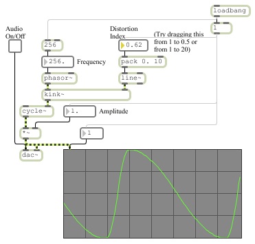
Phase distortion is a synthesis technique that was used in some Casio synthesizers in the 1980s. In traditional wavetable synthesis, a linear upward ramp signal is used as a phase index to read cyclically through a wavetable containing a particular waveform (a sine wave being the most common). In MSP you can do that by connecting the output of a phasor~ object, which generates a cyclic upward ramp from 0 to 1, to the right (phase offset) inlet of a 0 Hz cycle~ object (containing one cycle of a cosine waveform by default). However, the kink~ object distorts the linear ramp of phasor~, putting a bend (a.k.a. a "kink" or "knee") in it at a designated point. When that distorted ramp is used to read through the waveform in cycle~ the result is a distorted sinusoid that has more harmonic content as the distortion (the sharpness of the bend in the ramp) becomes more severe. Thus the harmonic content of the output varies dynamically as the bend point of the kink~ object changes. This patch allows you to vary the bending effect of the kink~ object, and see and hear the effect.
April 29, 2010
Example 31: Invert the pitches of MIDI notes.
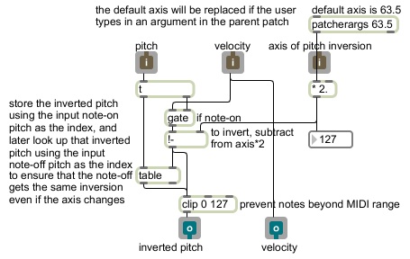
To invert a musical phrase around a particular axis of symmetry, multiply the axis pitch by 2, then subtract the played pitches from that. For example to invert all pitches around the axis of middle C (MIDI key 60), you would subtract the pitches from 120.
When modifying the pitch of MIDI notes like this, you need to take care that the note-off message gets the same modification as the note-on message did, in order to make sure that the note gets turned off properly. The most reliable way to do that is to store the modified pitch associated with the unmodified pitch, and then look up the modification when the note-off message arrives. The table object is good for storing indexed values and looking them up later, so that's what's used in this example. Another good example of this, with a detailed explanation, is provided Example 21 from last year's class, which handles note transposition in a very similar way.
When the axis of pitch symmetry is specified, it is multiplied by 2.0 and stored in the right inlet of a !- object. (Notice that we use a float multiplication so as to permit the specification of pitch axes that are precisely between two notes by using a .5 fractional part. For example, to specify an axis between E and F above middle C, one would use 63.5. That also happens to be exactly in the middle of the range of possible MIDI pitches, so it's what we use as a default value if the user does not type in any argument in the parent patch.)
This patch shows the use of the patcherargs object instead of a #1 argument. This allows us to specify default values for arguments, which will be sent out the left outlet of patcherargs as soon as the patch is loaded, but which will be replaced by any arguments that the user types in when the patch is used as an object in another patch. If the user does not type in any argument, the specified default value will be used.
When a pitch and a velocity come in, the velocity (which should come in first) is used to determine whether to open a gate to pass the pitch to the inverter. If it's a note-on, the pitch will get inverted and also will get stored in the table with the incoming pitch as its index. If it's a note-off, nothing will get through the gate, but the pitch will still be used to look up the previously stored inverted pitch and send that out.
Finally, since this inversion process could potentially flip the pitch outside of the 0-127 range, we use a clip object to restrict the output pitches within that range.
Example 32: Try out the invertpitch subpatch to invert the pitches of MIDI notes.
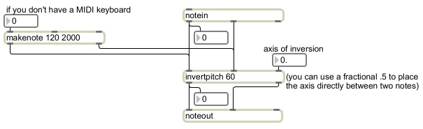
This is an example patch you can use to try out the invertpitch patch shown in Example 31. Of course, you will first have to download the patch from Example 31 above and save it with the name "invertpitch".
Example 33: Delay MIDI note messages.
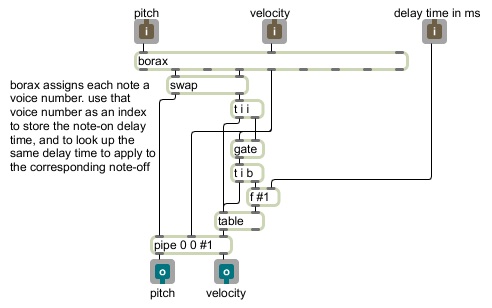
To delay a single bang message by a certain amount of time, use the delay object. But to delay any other sort of message -- a number, a list, even a group of different messages -- use pipe. The pipe object dynamically allocates memory as it stores more and more messages, so it can keep track of many messages at once, even if they arrived at different times and have different delay times (unlike the delay object, which can only hold one bang at a time).
This patch uses pipe to delay pitch and velocity values, so it functions as an adjustable delayer of MIDI notes. When delaying MIDI note messages like this, you need to take care that the note-off message gets the same delay as the note-on message did, in order to make sure that the note gets turned off properly. For example, imagine what would happen if the delay time were made considerably shorter before the note-off message arrived. The note-off might actually get sent out before the corresponding note-on, resulting in a stuck note. The most reliable way to ensure that the note-on and the note-off get the same delay time is to store the delay time that was applied to the note-on, and then look up that delay time when the note-off message arrives. The table object is good for storing indexed values and looking them up later, so that's what's used in this example.(Example 31 above shows a similar technique, using the note-on pitch value as the index.)
The incoming pitch and velocity values go to a borax object, which generates a unique "voice number" for each note it receives. The voice number comes out after the pitch and velocity values, but the pitch value and the voice number both go to a swap object, which swaps the message order so that the voice numbers goes out the right outlet first, and then the pitch goes out the left outlet. In the case of a note-on message, the velocity value opens a gate, and the voice number goes through the gate, bangs the f object holding the delay time, and stores the delay time in the table using the voice number as the index. It then sends that delay time to the right inlet of pipe. The velocity and pitch values thus get delayed that amount of time by pipe. In the case of a note-off, nothing gets through the gate, but the voice number is still used to look up the delay time for that note, so that the note-off velocity and pitch will be delayed the same amount of time by pipe. The number of inlets the pipe object has is determined by the number of initializing arguments that are typed into it. It can delay any type of items (int, float, or symbol), depending on the argument. There should be one argument for each inlet, plus a final argument specifying the delay time. In this example, the delay time in the f object and in pipe is #1, which will be replaced by the typed-in argument when this patch is used inside another patch, or which will be 0 if nothing is typed in.
Example 34: Try out the delaynote subpatch to delay MIDI note messages.
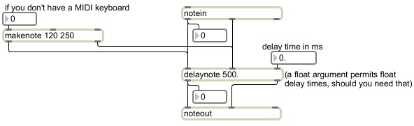
This is an example patch you can use to try out the delaynote patch shown in Example 33. Of course, you will first have to download the patch from Example 33 above and save it with the name "delaynote".
May 11, 2010
Example 35: Multi-tap audio delay with feedback.
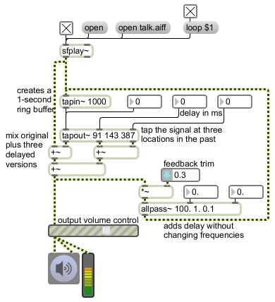
Audio delay is achieved by creating a buffer in which the most recent past sound can be stored. Usually this is called a "ring buffer" or "circular buffer", because when the buffer is filled (with, let's say, the past one second of sound), it loops around and begins refilling itself at the beginning, thus overwriting the sound that was stored more than one second ago. In this way, the buffer always stores the most recent one second (or whatever amount can be contained in the buffer), and we can access past sound samples by working backward through the buffer from the most recently stored sample (looping back to the end and continuing backward if necessary). But in MSP you don't really need to worry about the inner workings of such a circular buffer, because the object tapin~ takes care of that for you. The tapin~ object creates a circular buffer space in memory to store the designated amount of its most recently received audio signal.
The tapout~ object, once its inlet is connected to the outlet of a tapin~ object, can access ("tap") that stored signal at any point in the recent past (up to the maximum time stored in the tapin~). The tapout~ can tap the signal at as many points as it has typed-in arguments. (It always has at least one tap point, by default.) The delay time(s) are specified in milliseconds, either by the typed-in argument, by a float or int received in the inlet, or by a signal received in the inlet. (As is the case with all MSP objects, if an inlet can receive either a signal or a float, if it has a signal connected to it, then arguments and floats are ignored.)
In this example, the tapout~ object has three different delay times specified by typed-in arguments, and those delay times can be changed with numbers in its inlets. The outputs of tapout~ are mixed with (added to) the original undelayed signal, sent to a gain~ object to control their volume (since the sum of the four signals could easily exceed 1) and then sent to the ezdac~. The output(s) of tapout~ can be fed back into the inlet of a tapin~ to create feedback. The minimum delay time that can be obtained with tapout~, however, is the duration of one signal vector. The fed-back signal will (must) always have at least that much delay. Also, in order to avoid clipping due to rapidly-accumumlated additions, it's almost always a good idea to scale down the delayed signal -- by multiplying it by some number between 0 and 1 -- before feeding it back into the tapin~ from which it came.
In this example, the fed-back signal is also passed through an all-pass filter (allpass~). This type of filter has the effect of delaying different frequencies by slightly different times, thus changing their phase relationships, without altering the frequency content of the sound. In audio it can be used to reduce or blur resonance effects caused by feeding sound back with short delay time.
Example 36: Flanging.
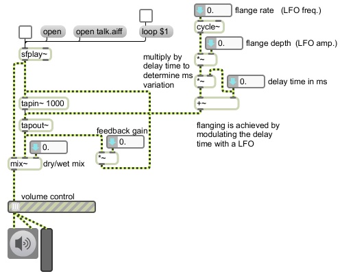
For this example to work properly, you will also need to download the additional Max file mix~.maxpat. That patch is identical to the patch described in Example 20 from the 2009 class examples.
The audio effect of "flanging" is achieved by using a LFO to continually modulate the delay time of a sound, and then (usually) mixing the delayed sound with the original sound to create interference. Modulating the delay time of a sound has the effect of changing its virtual distance from the listener, thus creating a subtle (or not-so-subtle) Doppler effect.
To modulate the delay time without creating clicks, the delay time of tapout~ must be supplied as a smoothly-changing signal. A sinusoidal cycle~ object is the most common LFO source. Its amplitude must be scaled so that it produces the range of millisecond delays desired (i.e., the desired plus-and-minus range of milliseconds by which the delay time will fluctuate), and then that value must be added to a base delay time within the delay buffer. In this example, the amplitude gain of the LFO (i.e., the modulation depth) is first limited from 0 to 1, and then is multiplied by the base delay time. Thus, the modulation depth is specified as a fraction (0 to 1) of the delay time. Specifying a longer delay time will proportionally increase the modulation depth.
Using a relatively short delay time, a moderate modulation depth, a very slow modulation rate (less than 1 Hz), and a balanced dry/wet mix, you can achieve subtle flanging effects. Increasing the flange rate to several cycles per second can make a sort of flanging tremolo effect. And of course, by increasing the delay time, modulation depth, modulation rate, and wetness, you can create a wide range of surreal effects. Feeding some of the flanged signal back into the delay line further complicates the effect.
Example 37: Chorusing.
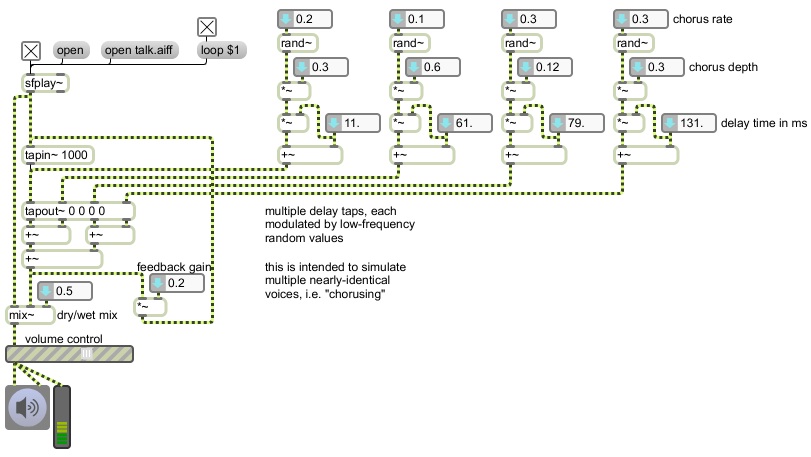
For this example to work properly, you will also need to have downloaded the additional Max file mix~.maxpat. That patch is identical to the patch described in Example 20 from the 2009 class examples.
The audio effect called "chorusing" is derived from the natural phenomenon of interference that occurs when multiple instruments or voices play (imperfectly) in unison. There are constant unpredictable irregularities in timing and tuning between the ostensibly unison voices, causing subtle random types of interference. The chorusing effect is achieved similarly to flanging, usually with the following differences:
- the delay times are usually greater than 20 milliseconds, to simulate the kind of timing imperfections evident in human performance,
- delay times are often modulated with a Brownian (low-frequency) noise source rather than a sinusoidal oscillator, the better to simulate random mistunings of human playing, and
- more than one delay tap is often used, in order to simulate multiple voices.
In this example, four delay taps are modulated by very-low-frequency noise from rand~ objects. The scaled delayed signals can be fed back into the tapin~ for more complexity (emulating still more voices). The delayed signals are mixed with the original, scaled by gain~ and sent on to the ezdac~. For such an effect to be easily controllable, one should really have a scheme that allows the user to adjust all of the modulators with just one or two dials. One could also consider panning each of the delayed "voices" to a different virtual location in the stereo field before sending the mixed sound out.
May 13, 2010
Example 38: Basics of drawing in the lcd object.
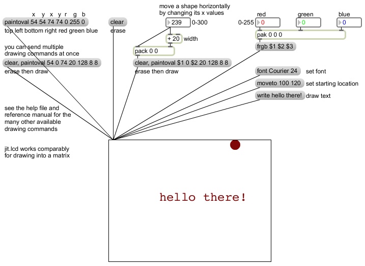
Onscreen drawing of lines, shapes, text, and stored images is done using drawing commands derived from Apple's QuickDraw/Quartz systems for creating 2D graphics. The lcd object understands many such commands, and can serve as a 2D drawing surface (and/or animation stage) within a Max patch. Note that almost everything that can be drawn in the lcd object can also be drawn into a Jitter matrix with the jit.lcd object. Once the drawing exists in a Jitter matrix, it can be mixed or composited with other video images and can be displayed in a separate window (or fullscreen) with jit.window.
This patch demonstrates a few basic drawing commands. The drawing location is always specified as x,y coordinates relative to the top-left corner of the lcd. So, for example, to begin drawing at a point 100 pixels to the right of, and 120 pixels down from, the top-left corner of the object, you would specify a location "100 120". Colors are almost always specified as three numbers from 0-255, which are "RGB" values expressing the relative intensities of light in the three primary light colors red, green, and blue. In this example, you can see that bright green is described by "0 255 0" (maximum green, but no red or blue), and dark red is described by "128 8 8" (medium amount of red, but almost no green or blue).
The message frgb is used to specify a default foreground color for the lcd, which is the color that will be used whenever no color is specified for a drawing command. (The message brgb is used to specify a background color for the stage, which will be used whenever the stage is erased with a clear message.) There are so many possible command messages that it's impractical to try to discuss them all in examples. You need to read the documentation and experiment in order to understand all of the capabilities of lcd and jit.lcd.
Example 39: Drawing an image from a file into lcd.
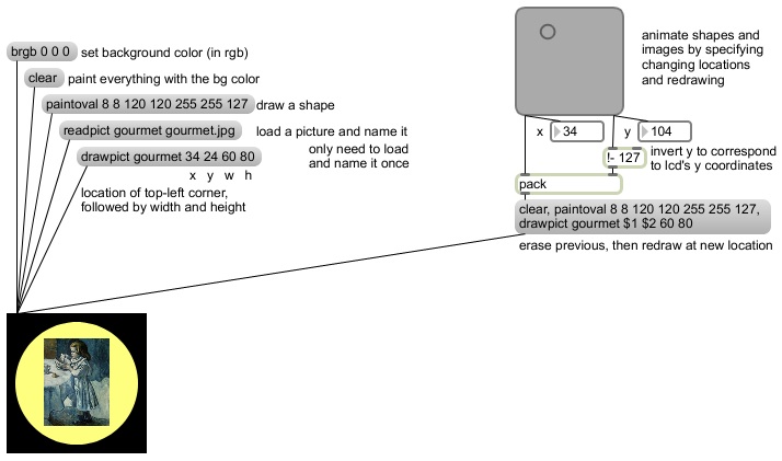
For this example to work properly, you will also need to download the small image file gourmet.jpg.
To draw a previously-saved image in lcd, you need to tell the lcd the name of the file you want to read in (which, of course, must be located in Max's search path) and you need to choose a name by which you want to refer to that image. You do this with the readpict message, in which you include your own (arbitrary) name and the name of the file. Once you have done that, you can draw that image using the drawpict <imagename> message, in which you can optionally include the desired x and y location offset as well as width and height specifications to resize the image.
Example 40: Drawing with sprites in lcd.
![]()
For this example to work properly, you will also need to download the small image file guitariste.jpg.
In order to manage the drawing and redrawing of multiple items that might be moving independently in complex ways, lcd uses the animation concept of "sprites". A sprite is a specified drawing (which really could be of any degree of complexity) that is treated as an independent object. When the sprite is called by name, a single command can draw the sprite at a desired location and also take care of re-drawing the stage in the area that the sprite used to occupy.
In lcd, the message recordsprite allows you to start describing a sprite. Subsequent drawing messages describe the sprite. Then the message closesprite <spritename> stops recording the description and stores the description with the associated sprite name. After that, you can draw a unique instance of that sprite with the message drawsprite (with optional x and y offset to specify its location).
Although it's not visible to you, in the Inspector for the pictslider object, the output ranges have been set to correspond to the range of values that are appropriate for the lcd object. The minimum and maximum for the y value output range have been exchanged so that the direction of the y values coming out of pictslider correspond to the direction in which lcd expects them.
The order in which sprites are drawn onscreen (which will determine their front-to-back ordering and thus their occlusion characteristics) is initially determined by the order in which the sprites were recorded. However, you can send sprites to the front or back of that ordering with the messages frontsprite <spritename> and backsprite <spritename>. Experiment with the frontsprite and backsprite messages in the example patch to see their effect on the drawing order of the sprites.
Note that sprites are not implemented in jit.lcd. That's primarily because in Jitter the drawing commands all take place offscreen in the jit.lcd object's matrix, and are only displayed when the object sends out its matrix to a jit.window or jit.pwindow. So the expectation is that you, the programmer, will send the proper messages to draw the entire image the way you want it to be seen, and then send a bang to output the jit_matrix message. All of that must happen for each frame you wish to display.
Example 41: Simple subtitles in a video.
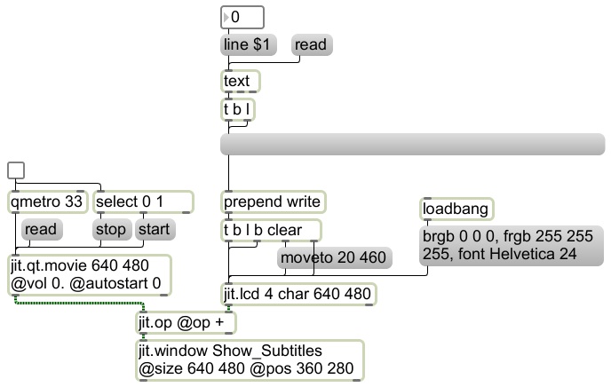
For this example to work properly, you will also need to download the small text file subtitles.txt.
Because of the ease with which one can draw text in lcd, using the jit.lcd object is a very easy way to include subtitles, credits, or any other sort of text in a video displayed in Jitter. The text can be drawn with a simple write message, and the contrast between the text and the background can be used to mask the text and non-text portions of the matrix.
There are various ways one could do the compositing (for example, using jit.chromakey or jit.alphablend), but this example shows a very efficient and straightforward way to composite text and image with a simple addition operation. The background color is made black (RGB values "0 0 0" and the foreground color is made white (RGB values "255 255 255"). The text is thus written in white on a black background. When that matrix is added to an image, all of the cells with values of "0" leave the video image unchanged, and all the cells with values of "255" push those pixels to their full white value.
The text in this case is supplied by reading lines of text from a text file with the text object. The text object prepends the word "set" before its output (with the intention that you will use the text to set the contents of another object such as message box), so you need to either strip off the word "set" with a route set object, or, as we've done here, first set the contents of a message box and then bang it to send it out. To draw the text in jit.lcd you then just need to prepend the word "write" before the text.
Note that for each new line of text, we need to clear the lcd (filling all its cells with 0), move the pen to the desired location, write the text, then send out the contents of the matrix. That matrix will then be added to each frame of video coming from the jit.qt.movie object.
May 18, 2010
Example 42: Simple demonstration of the transport object.
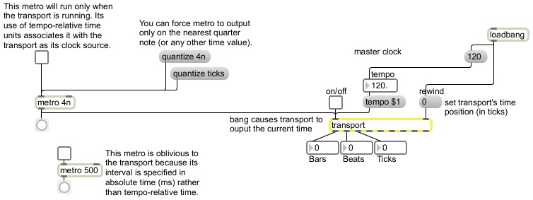
Timing objects such as metro normally operate with their time interval specified in milliseconds, and they are controlled by the Max scheduler, which is always running. You can alternatively specify timing using tempo-relative time units such as rhythmic note values or bars, beats, and ticks, in which case the timing object will be controlled by a global master clock called the "transport", which can itself be easily started and stopped via the transport object. The transport relies on those more music-oriented timing units such as bars, beats, and ticks (480ths of a quarter note), the absolute millisecond duration of which actually depends on the tempo (beats per minute) and the time signature that have been assigned to the transport. (By default, the tempo is 120 beats per minute and the time signature is 4/4.) Timing objects that use tempo-relative time units only run when the transport is running.
In the example patch, try starting the two metro objects. The one that uses millisecond timing always works, whereas the one that has its time interval specified as a quarter note only works when the transport object is turned on.
When the transport object receives a bang in its left inlet, it sends out information about the current state of the transport such as its tempo, time signature, and current time. The transport is always at some clock time. Even if you never use a transport object, the transport still has a default tempo (120 bpm), time signature (4/4), and a time of "1.1.0" (bar 1, beat 1, and 0 ticks) a.k.a. "0 ticks". By connecting the outlet of a metro to the left inlet of transport, you can get regular reports of the current time of the transport.
Notice that, unless you turn on the transport and the metro at exactly the same instant, it's likely that metro will be offset from the transport's beat by some number of ticks. However, you can use the metro's quantize attribute to specify a grid to which it must snap its output. For example, sending it the message quantize 4n will cause it to send its output only at times that are exactly on the transport's quarter-note beat.
Example 43: Other basic functionality of the transport object.
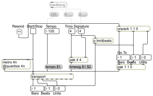
This patch does some of the same things as the "GlobalTransport" patch in the Extras menu, and shows what is likely going on behind the scenes in that patch. The toggle labeled "Start/Stop" starts the transport and immediately turns on the metro to begin triggering time reports. The button labeled "Rewind" sends a time position of bar 1, beat 1, 0 ticks to the transport to reset its time. You can enter any time you want in the number boxes labeled "Bars", "Beats", and "Units". The tempo <bpm> message sets the transport's tempo attribute. The timesig <numerator> <denominator> message sets the time signature. Although it's not visually obvious, the numerator is actually specified in this patch with a umenu (in Scrolling mode so that it responds to dragging with the mouse) that contains only numbers that are powers of 2. The numerator and denominator both go to a pak object, and then become part of a timesig message. (pak differs from pack in that it sends its output whenever it receives input in any inlet, whereas pack sends its output only when it receives input in its left inlet.) When a numerator is specified, it also is used to set the maximum of the "Beats" number box. (Double-click on the p limitbeats object if you want to see how that's being done.)
Example 44: The translate object updates its output when the tempo changes.
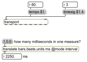
The translate object converts a message from one type of time unit to another. It uses the tempo and the time signature of the transport to do that calculation. If the tempo or the time signature changes, the result of the calculation would be different, so translate always resends its output whenever the transport receives a change to one of those values.
A time message of bars-beats-units, such as "1.1.0", can potentially mean either of two things. It can mean a time position of the transport -- an instant in time -- such as "the first beat of the first bar" or it can mean a time interval -- a duration of time between two positions -- such as "one bar plus one beat's worth of time". When translated into some other time unit such as ticks, these two possibilities might not yield the same result. The time position at the first beat of the first bar is 0 ticks, but the duration of one beat plus one bar (assuming a time signature of 4/4) would be 2400 ticks (1 bar + 1 beat = 5 quarter notes = 480 x 5 ticks = 2400 ticks). Therefore, the translate object can operate in either of two modes -- position mode or interval mode -- determined by its mode attribute. In this example we're trying to find the duration of one measure, so we have explicitly set the mode attribute to "interval".
Example 45: Tempo-relative timing for MSP LFO control.
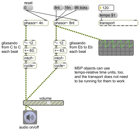
The MSP phasor~ object is frequently used as a low-frequency control signal for audio. Because it is often used to control other signals over a specific period of time, phasor~ can use tempo-relative timing, too. The frequency (rate) of a phasor~ is normally specified in Hertz, but you can alternatively give phasor~ a time interval, using tempo-relative time units, and it will use the inverse of that to determine its frequency.
For example, if I wanted a phasor~ to ramp from 0 to 1 every 500 milliseconds, I would specify a frequency of 2 Hz so that it will complete one cycle every 1/2 second. I could alternatively give it a tempo-relative time unit, such as 4n, which -- if we assume the default transport tempo of 120 bpm -- equals 1/2 second (500 ms), and phasor~ will interpret that as its period, and use the inverse of that (2/1) to determine its frequency. If the tempo of the transport changes, phasor~ will revise its frequency accordingly. This works even if the transport is not running.
In this example patch, phasor~ is being used to control a pitch glissando of one octave, which then gets translated by mtof into frequency for a cycle~ object. The phasor~ on the left completes one sweep per beat, while the phasor~ on the right completes three sweeps per beat (once for each eighth-note triplet). If you change the tempo of the transport, the phasor~ objects adjust their frequency to match the new tempo, thus staying in sync. If you provide the phasor~ on the right with a new time interval -- a sixteenth note or a quintuplet sixteenth note (which equals 96 ticks) -- it will change its rate. Unless that change were to happen exactly on the beat, though, the phasor~ on the right will likely no longer be in phase with the phasor~ on the left. So if you want them to remain in phase it's a good idea either to trigger such a change exactly on the beat or to reset the phase of both phasor~s by sending a phase value in their right inlets.
Other MSP objects don't understand tempo-relative time units the way that phasor~ does, but there's usually a way to sync them to the transport's tempo if you want to. For example, if you want use tempo-relative timings for the rate of a cycle~ object that you're using as a LFO, you can just set the frequency of the cycle~ to 0, and then drive it by connecting the output of a phasor~ to its right inlet. If you want the delay time of a tapout~ object to be exactly the same interval as a tempo-relative time unit, you can use translate to convert that time unit into milliseconds.
Example 46: Synchronizing MSP audio loops with the transport.
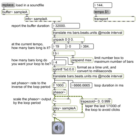
This example shows one way you might use phasor~ to make the length of an audio sample loop stay precisely synchronized with the beat of the transport.
Upon loading a sound file into a buffer~, you can use info~ to learn the duration of that buffer~ (which will be the same as the duration of the sound file if you used the replace message to load it in), and then translate that duration into bars.beats.units to find out how many measures long it is at the current transport tempo. In this example, the number of bars is used to set the maximum limit of a number box. You can use that number box to specify how many bars of the sound file you'd like to play in a loop. That number of bars is translated back into milliseconds to determine the rate and range of a phasor~. The phasor~ drives a play~ object to read from the buffer~, and it also drives a trapezoid~ object which is used as an amplitude envelope to taper the last 1/1000th of the loop in order to avoid clicks.
As you change the tempo of the transport, translate will update its output, and the phasor~ will therefore continue to read the correct number of bars' worth of sound from the buffer~.
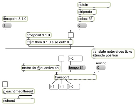
Example 47: Using timepoints for interactive sequencing.
The timepoint object sends out a bang when the transport reaches a specified time position. This can be useful for causing something to happen -- or for starting an entire process -- at a particular instant during the transport's progress. A timepoint might, for example, even trigger a new time position value to be sent to the transport object itself, thus causing the transport to leap to a different time.
In this example, when the transport reaches the downbeat of measure 8, the timepoint 8.1.0 object triggers the number 1, which gets stored in the right inlet of the if object and also turns on the note-playing algorithm encapsulated in the p eachtimedifferent object. When the transport reaches the downbeat of measure 9, the timepoint 9.1.0 object triggers the if object either to set the transport back to time position 8.1.0 (if the value in the right inlet of if is 1) or to turn off the note-playing algorithm instead and allow the transport to proceed (if the value in the inlet of if is 0). In effect, this creates a loop in the transport, cycling repeatedly through measure 8 until 0 comes in the right inlet of if, which will allow the transport to proceed beyond the downbeat of measure 9.
The 0 in the right inlet of if is triggered when the MIDI note 55 (G below middle C) is received (or, of course, by clicking on the message box or the toggle). This shows how the transport can actually be controlled interactively by a performer. You could think of this patch as telling the transport to repeat a 1-measure "vamp" in measure 8 until a G below middle C is played, at which point it can continue forward. And since the downbeat of measure 8 re-triggers the note-playing algorithm to choose a whole new set of random numbers -- specifying rhythmic value, velocity, base pitch, and pitch range -- each time, each pass through measure 8 sounds different.
Example 48: Multiple simultaneous tempi using named transports.
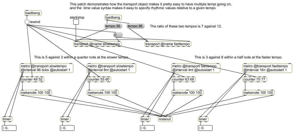
One of the most intriguing features of the transport object is that there can be multiple independent transports in action at the same time. If a transport object has not had its name attribute set, it refers to the one global transport. However, you can create an independent transport by giving the transport object a name (i.e., by setting its name attribute to some name of your choice). You can then cause any other timing object to refer to that transport by setting the object's transport attribute to be the same as the name of the named transport.
For example, in this patch there are two transport objects, one named "slowtempo" and one named "fasttempo", and their tempos have been set to be 56 bpm and 96 bpm respectively. The two metro objects on the left refer to the "slowtempo" transport for their timings, and the two metro objects on the right refer to the "fasttempo" transport. To further complicate matters, each metro is using a different rhythmic value as its time interval. From this example it should be clear that named transports make it easy to create music that is polymetric, polyrhythmic, and that even has multiple simultaneous tempi governing different streams of rhythmic activity.
May 25, 2010
Example 49: Play random clips (in reverse) from a RAM buffer.
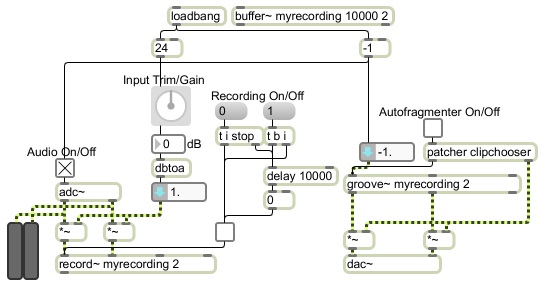
This example demonstrates creating a RAM buffer to hold a 10-second stereo recording, recording live audio into it (with input volume adjustment), and then playing randomly chosen backward clips of that sound, with a trapezoidal window to taper the beginning and ending of each clip to avoid clicks.
The clipchooser subpatch randomly chooses a clip duration from 1 to 2000 milliseconds, uses that duration to create an amplitude envelope of the proper duration, then chooses a starting location in the buffer (making sure that the location is not so early in the buffer that it would prevent the backward clip from completing), and sends out the amplitude envelope and the starting time. (Note that this subpatch assumes that the rate of the groove~ object is -1.) It delays for that duration (using delay) before repeating the process to choose the next clip.
This page was last modified May 27, 2010.
Christopher Dobrian
dobrian@uci.edu