Example 1: Score following with the follow object
This page contains examples and explanations of techniques of interactive arts programming using Max.
The examples were written for use by students in the Music Technology course at UCI, and are made available on the WWW for all interested Max/MSP/Jitter users and instructors. If you use the text or examples provided here, please give due credit to the author, Christopher Dobrian.
There are also some examples from the previous classes available on the Web: examples from 2012's Interactive Arts Programming class, examples from 2011's Music Technology class, examples from 2010's Interactive Arts Programming class, examples from 2009's class, examples from 2007's class, examples from 2006's class, examples from 2005's class, and MSP examples and Jitter examples from 2004's class.
While not specifically intended to teach Max programming, each chapter of Christopher Dobrian's algorithmic composition blog contains a Max program demonstrating the chapter's topic, many of which address fundamental concepts in programming algorithmic music and media composition.
You can find even more MSP examples on the professor's 2007 web page for Music 147: Computer Audio and Music Programming.
And you can find still more Max/MSP/Jitter examples from the Summer 2005 COSMOS course on "Computer Music and Computer Graphics".
Please note that all the examples from the years prior to 2009 are designed for versions of Max prior to Max 5. Therefore, when opened in Max 5 or 6 they may not appear quite as they were originally designed (and as they are depicted), and they may employ some techniques that seem antiquated or obsolete due to new features introduced in Max 5 or Max 6. However, they should all still work correctly.
[Each image below is linked to a file of JSON code containing the actual Max patch.
Right-click on an image to download the .maxpat file directly to disk, which you can then open in Max.]
Examples will be added after each class session.
April 3, 2012
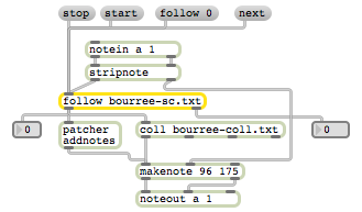
Example 1: Score following with the follow object
This patch is based on an example in the Max 2.0 Tutorial, chapter 35. It demonstrates score following using the follow object. For it to work properly, in addition to saving the patch itself, you will need to save these two text files, using the same file names as are shown here -- bourree-sc.txt and bourree-coll.txt -- in the Max file search path.
The patch is explained in these pages extracted from the original Max Tutorial. Note that I have changed what was a funbuff object in the original file into a coll object for this example. That made the patcher "silencer" referred to in the text unnecessary, so you don't see it in this example patch.
Read in the score file of the Bach bourree melody and listen to it. Then click on the 'follow 0' message box above the follow object; that causes the follow object to start following you from the beginning of the score. Play the melody on your MIDI keyboard, and Max will play the left hand accompaniment. [N.B. The seq and follow objects can read any MIDI file that is in "format 0" (i.e., with all data on a single 'track').]
April 10, 2012
Example 2: Some objects for generating numbers
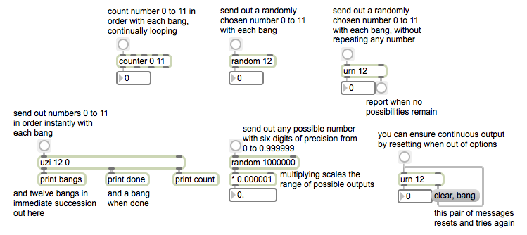
This patch shows four objects that are useful for generating numbers, each with a different behavior. The arguments to these objects determine how many different possible numbers the object will generate, and the range of those numbers. The range can be changed, though, by 'scaling' (multiplying) them and/or by 'offsetting' (adding something to) them.
Example 3: Controlling the range of a set of numbers
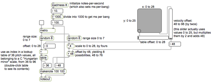
This patch is intended to show how to generate any desired range of numbers by some combination of the following operations: 1) generate a set of possible numbers with one of the number-generating objects shown in the previous example, 2) optionally scale the size of the range by multiplying all the numbers by a common factor, 3) optionally offset the range by adding a certain amount to each of the numbers, 4) optionally use those numbers to look up a stored set of desired results.
In this case, we're accomplishing a specific task with that method. We're playing randomly chosen notes within one octave (8 notes) of a particular scale, at one of 8 randomly chosen possible loudnesses (within a certain dynamic range), and we're able to control the pitch and loudness ranges with the mouse.
The millisecond interval of the metro determines how often the notes are played, and we use the same number of milliseconds to control the duration of the notes. To express that note rate in terms of notes per second, we just divide the notes per second into 1000 to convert it to milliseconds per note.
For pitch, we generate random numbers 0 to 7, add some number (from 0 to 28) to that, and then use that as an index to read from a table (array) of 36 possible pitch values. We entered the desired pitch values into the array by typing them as text and pasting them into the table. So, the range of randomly chosen indices is always just 8 possibilities (the random numbers 0 to 7) but we can use those to access any part of the table by offsetting them; the offset can be anywhere from 0 to read from the lowest part of the array (indices 0 to 7) up to 28 to read from the highest part of the array (indices 28 to 35).
We want to do something similar for the note velocities. In this case, the precise velocities are not so important as that they be within a desired range -- low velocities for softer notes and high velocities for louder notes. So the actual math we do for the velocities is somewhat arbitrary, but it does illustrate the control of range, scale, and offset. We choose a range of random numbers 0 to 7. We multiply that by 4 so that the numbers now go by fours from 0 to 28; thus there will always be 8 possible velocities, but always within a range that's constrained so that the difference between the maximum and the minimum is 28. We add an offset that's variable between 48 and 98; so when the offset is at its lowest we get velocities from 48 to 76, and when the offset it at its greatest we get velocities from 98 to 126.
The slider object is handy in this regard because you can do scaling and offsetting within the slider by setting its 'mult' (multiplier) and 'min' (minimum) attributes in the Inspector. The velocity slider actually just goes from 0 to 25, but internally that gets multiplied by 2 and has 48 added to it, so the output of the slider actually goes by twos from 48 to 98.
But what if we want to control both pitch and velocity with the mouse at the same time? The pictslider object is a two-dimensional user-interface slider, which sends out both x and y coordinates of the slider's position. Here we have set its x axis to go from 0 to 28 for the array index offset, and we have set its y axis to go from 0 to 25 for the velocity slider (which will translate that into a velocity offset from 48 to 98). Set the note rate you want, turn on the metro with the toggle, then drag on the pictslider to hear the change in pitch range and velocity range.
Example 4: Oscillators controlled by cellular automata
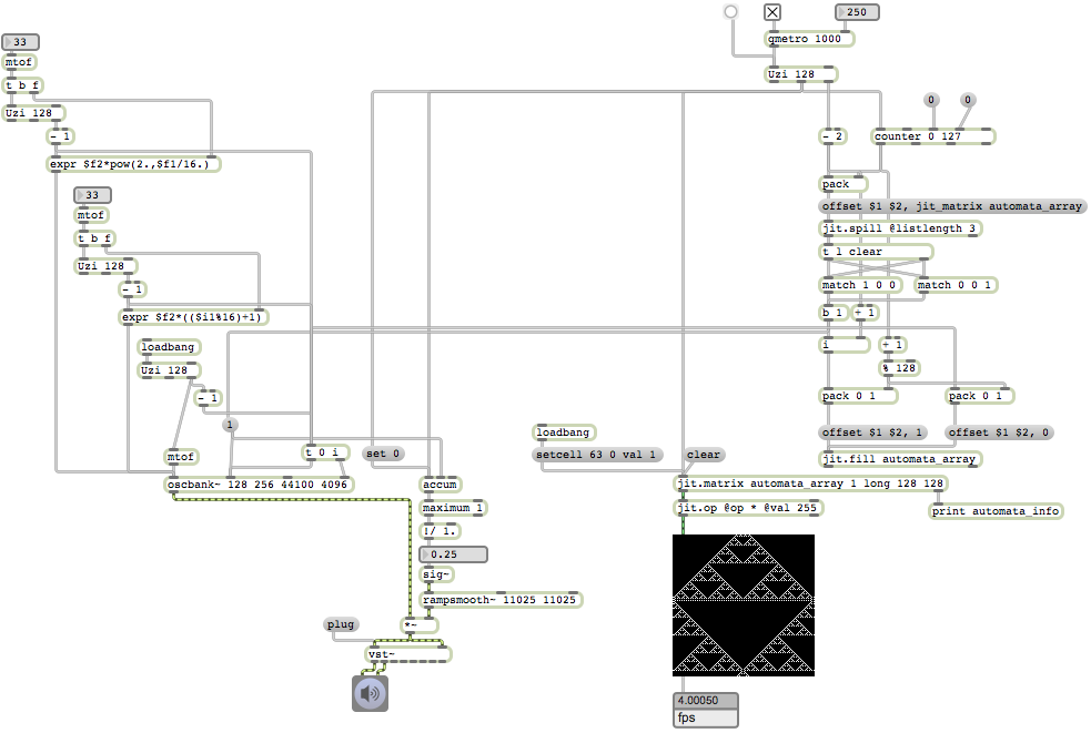
Relevant to the discussion of musical applications of cellular automata, here is a patch that controls a bank of 128 oscillators based on the on-off state of a row of cells in a Jitter matrix that is generated by some very simple rules of a cellular automaton.
I won't try to explain every detail of this patch, but will point to a few main features. The interval of the qmetro will determine how frequently the program reads a row of on-off states (1s or 0s) from a matrix, uses them to turn on or off oscillators in a oscbank~ object, and generates a new row of on-off states according to some simple rules (which are then visualized in the jit.pwindow object). The number boxes on the left are to choose the fundamental pitch of the oscillators. The number box on the top left produces 8 octaves of frequencies of a 16-notes-per-octave equal-tempered scale; the other number box tunes the oscillators to 16 harmonics of the fundamental pitch. The amplitude is adjusted in inverse proportion to the number of oscillators being played. If so desired, one can load a VST plug-in and run the sound through that for added processing.
Example 5: Algorithmic composition with math functions
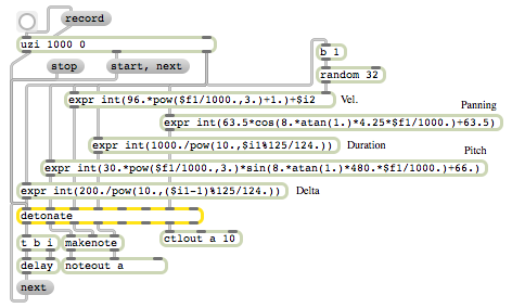
This patch is based on an example in the Max 3.5 Tutorial, chapter 44. It demonstrates a) the use of math functions to generate patterns for musical parameters and b) faster-than-realtime recording of MIDI data in the detonate object.
The detonate object is a multi-track MIDI sequencer. You can use it to record note information by sending it a 'record' message and then providing (in the first five inlets) vital MIDI note information consisting of delta time (the change in time from the onset of the previous note), pitch, velocity, duration, and channel. (You can also store ancillary information, such as controller data, along with each note event.) Then, to play that information back, you send detonate a 'start' message, followed by a 'next' message telling it to send out the next note. Because the time-till-the-next-note (i.e., the delta time of the next next note) comes out the left outlet, you can use that to determine how long to wait before sending the next 'next' message.
The uzi object will send out a fast-as-possible ascending series of numbers (and a bang for each one) in response to a single bang. In this example it instantaneously sends out 1000 numbers going from 0 to 999. Those numbers are plugged into various mathematical expressions to create specific functions (curves or shapes) over the course of 1000 notes. That information is recorded by detonate as note information, and when uzi is done it triggers 'start' and 'next' messages to begin playing the notes.
The effect of those expressions is described in two pages from the Max 4.6 Tutorial manual. (Note, the manual refers to a -1 object after the right outlet of uzi, an object which existed in the original because uzi could originally only count starting from 1. In more recent versions, uzi can be instructed to start counting from any number, so we have set it to begin counting from 0, thus removing the need for the -1 object.)
April 17, 2012
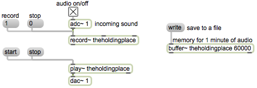
Example 6: Basic RAM recording into buffer~
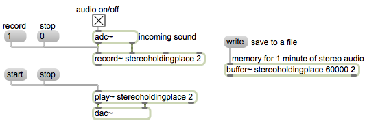
Example 7: Basic stereo recording into buffer~
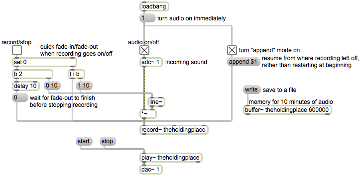
Example 8: Consecutive recordings concatenated in the same buffer~
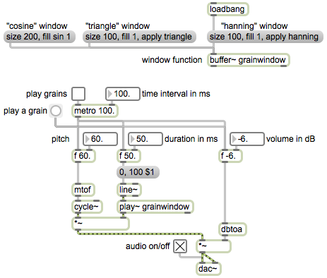
Example 9: Single stream of sine grains
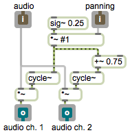
Example 10: Constant-intensity panning subpatch
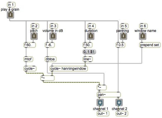
Example 11: Sine grain player suitable for use in poly~
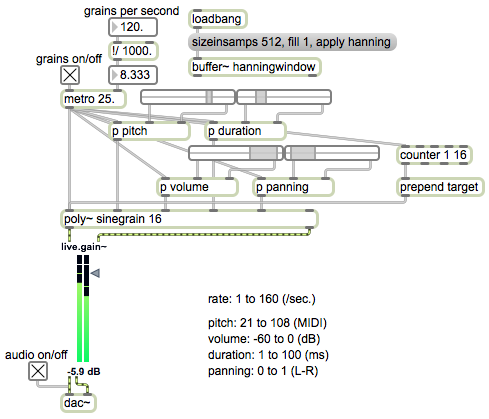
Example 12: Polyphonic granular synthesizer with parameter controls
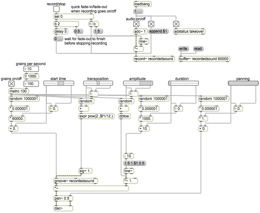
Example 13: Single stream of grains from a buffer~
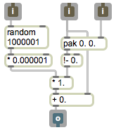
Example 14: Generate random numbers within a specified range
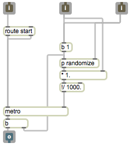
Example 15: Metronome with random perturbations of tempo
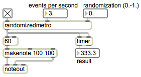
Example 16: Demonstration of the randomizedmetro subpatch
April 24, 2012
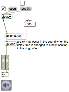
Example 17: Change of delay time may cause clicks
The main ways to delay a sound in Max are demonstrated in the examples from the previous quarter that show the delay~ object and the tapin~ and tapout~ objects. You might want to take a look at those examples and read the associated text to review how they work, and what their pros and cons are.
Whenever you change the delay time, you risk causing a click by creating a discontinuity in the output waveform. (The amplitude at the new location in the ring buffer is likely to be different from the amplitude at the old location, so the output waveform will leap instantly from the old amplitude to the new amplitude.) This patch allows you to try that, to confirm that clicks can occur. You might sometimes get lucky and change the delay time at a moment of silence thus avoiding a click, but the odds are that a click will occur. So if you plan to change the delay time while listening, you probably want to try to solve that problem. The next few examples will address the topic.
Example 18: Continuous change of delay time causes a pitch shift
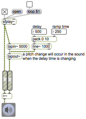
The way we commonly avoid clicks when changing the amplitude of a sound is to interpolate smoothly sample-by-sample from one gain factor to another, using an object such as line~. Does that same technique work well for making a smooth change from one delay time to another? As it turns out, that's not the best way to get a seamless unnoticeable change from one delay time to another, because changing the delay time gradually will actually cause a pitch shift in the sound.
This patch demonstrates that fact. When you provide a new delay time, it interpolates to the new value quickly; you'll hear that as a quick swoop in pitch. You can get different types of swoop with different interpolation times, but this sort of gradual change in delay time always causes some amount of audible pitch change. Of course there are ways to use this pitch change for desired effects such as flanging, but what we seek here is a way to get from one fixed delay time to another without any extraneous audible artifacts.
Example 19: Ducking when changing delay time
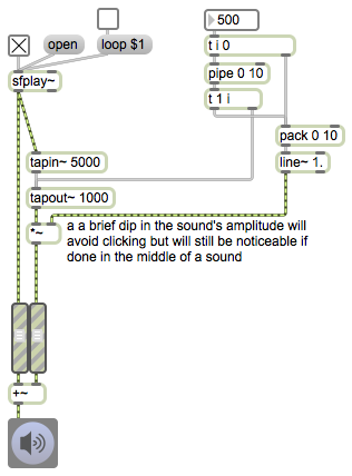
One possible solution to the problem of clicks occurring when delay time is changed is to fade the amplitude of the delayed sound to 0 just before changing the delay time, then fade back up immediately after the change. This does avoid clicks, but causes an audible momentary break or dip in the sound. This shows one way you could implement such momentary "ducking" of the amplitude. (The same idea with the delay~ object is shown in an example from the previous quarter's class.)
Example 20: Abstraction for crossfading between delay times
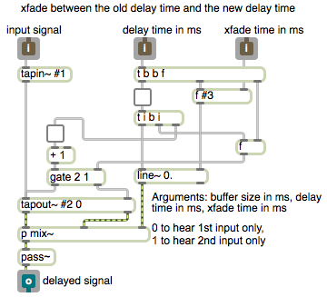
This example shows my preferred method for changing between different fixed delay times. It's an abstraction that I regularly use when I want a simple delay, and want the ability to change the delay time with no clicks or pitch changes. It's designed as an abstraction so that it can be used as an object (a subpatch) within any other patch.
It works by using two different delays of the same buffered sound, and crossfading between the two. The signal we want to delay comes in the left inlet and is saved in a tapin~ ring buffer that's connected to a tapout~ object with two delay taps (but we're initially only hearing the left output of tapout~, because the mix~ subpatch has the other signal of tapout~ faded down to 0). When a new delay time comes in the second inlet, it's directed to the inlet of tapout~ that's associated with the delay tap that's currently faded to 0, then fades up that signal while fading down the other. The third inlet allows for changing the crossfade time, so we can have quite sudden (nearly instantaneous, like 10 ms) changes of delay time that are nevertheless click-free, or we can have slower crossfades between delay times, even lasting several seconds (in which case we'll actually hear both delayed signals while we're crossfading between the two). By flipping back and forth between the two outlets of the gate object, and also fading back and forth between the two outputs of tapout~, we're always changing the delay time on the tap that is currently silenced. Try mentally stepping through the sequence of messages to understand exactly how this is accomplished.
Notice that this abstraction has been designed with the ability to accept typed-in arguments, so that its characteristics can be specified in its parent patch. The first argument in the parent patch will replace the #1 in this abstraction, so that the user can (indeed, must) specify the size of the tapin~ buffer. The second argument in the parent patch replaces the #2 to set the initial delay time of the object, and the third argument replaces the #3 to set the crossfade time that will be used for subsequent delay time changes.
N.B. There is actually a "screw case"--a way that this patch can fail to do its job correctly. If a new delay time comes in before the previous crossfade has finished, the tap that's being changed will still be audible, and we might hear a click. I haven't bothered to protect against this because I expect the user to know not to set a crossfade time that's longer than the expected minimum interval between changes of delay time. If we wanted to make this patch more "robust"--invulnerable to the screw case--we could refuse to accept a new delay time (or hold onto any new delay time) till the crossfade of the previous one has finished.
You can save this abstraction with a name such as delayxfade~ and try it out. (I try to use the convention of putting a ~ at the end of audio processing abstractions to remind myself that the abstraction involves MSP.)
Example 21: Demonstration of crossfading delay
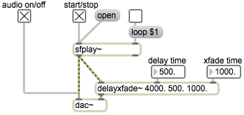
This patch demonstrates the use of the abstraction in the above example. It requires that you have saved that abstraction with the name delayxfade~.
Example 22: Abstraction for crossfading delay times of a remote tapin~ object
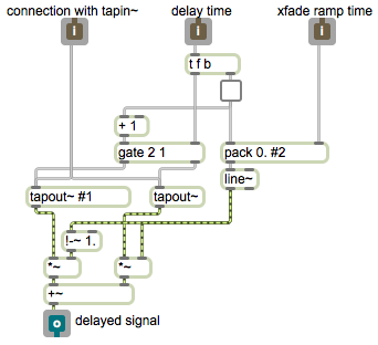
If we want to use the delay crossfading technique shown in the above example for multiple different delays of the same sound, the simplest solution is just to make multiple copies of that abstraction and send the same audio signal to each one. However, that's a bit inefficient in terms of memory usage because each subpatch would have its own tapin~ object, each of which would be containing the same audio data.
The way that tapin~ and tapout~ communicate is that when audio is turned on tapin~ sends out a 'tapconnect' message. When tapout~ receives a 'tapconnect' message it refers to the memory in the tapin~ object above it. So we really could modify our delay crossfade abstraction so that, instead of receiving an audio signal in its left inlet, it receives the message 'tapconnect'. That way, multiple copies of the abstraction could all refer to the same tapin~ object in their parent patch.
So this example shows a modification of the delay crossfading abstraction, in which the tapin~ object has been removed, and in which the left inlet expects a 'tapconnect' message instead of an audio signal. It will refer to a tapin~ object in the parent patch. You can save this abstraction with a different name, such as tapoutxfade~.
Example 23: Demonstration of multiple crossfading delay times referring to the same remote tapin~ object
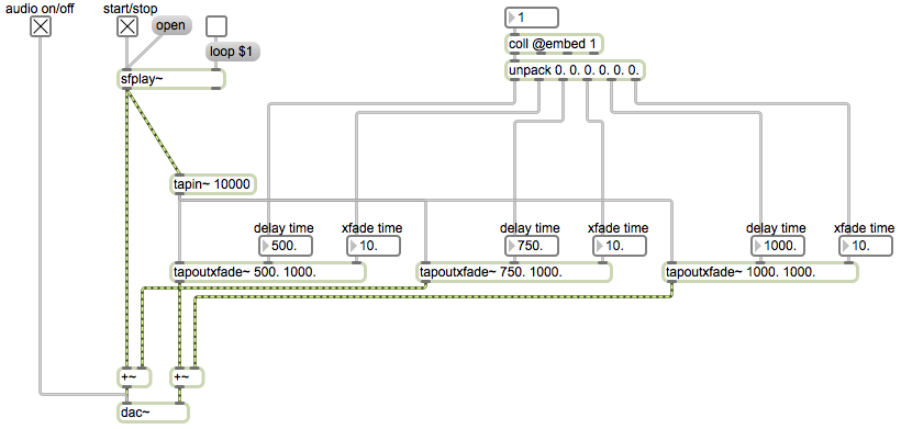
This patch requires the tapoutxfade~ abstraction in the previous example. When audio is turned on, the tapin~ object sends out the 'tapconnect' message to the three subpatches, thus associating their internal tapout~ objects with the same tapin~.
Example 24: Abstraction for constant-intensity stereo panning
For the basics of intensity panning for stereo sound in MSP, you might want to review Example 12 on linear amplitude panning, and Example 13 and Example 14 on constant power panning, from the 2012 Interactive Arts Programming class.
This patch is a very useful abstraction for constant-intensity stereo panning of sound. It's identical to Example 43 from the 2009 Interactive Arts Programming class, so you can read a description of it there.
Notice how this abstraction allows the user to specify the panning position in any one of three ways: as a typed-in value in the parent patch to set an initial value, as a float to change instantly to a new position, or as a signal to change continuously and smoothly from one value to another.
Save this patch with the name "pan~". It's needed for the next two examples.
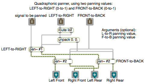
Example 25: Abstraction for quad panning using x,y coordinates
There are several standard and speaker configurations for 2-dimensional surround sound panning, such as quadraphonic (four speakers in a square or rectangular placement) and the 5.1 or 7.1 THX cinema surround specifications. There are also sound distribution encoding techniques that work for a variety of speaker configurations, such as the Ambisonics panning description, and there are processing techniques such as head-related transfer functions (HRTF) filtering.
This and the next few examples will show simple algorithms for intensity panning with a rectangular quadraphonic speaker configuration.
One way to implement two-dimensional panning is to specify the sound's virtual location as a x,y coordinate point on a rectangular plane representing the floor of the room, with a speaker at each corner of the plane. The x value can be used to represent the left-right panning (0 to 1, going from left to right) and the y value represents the front-back panning (0 to 1, going from front to back). For some purposes, simple linear panning might suffice (or even be found to be preferable). I usually prefer to use a constant intensity panning algorithm. So I use the pan~ abstraction to calculate the amplitudes that will provide the left-to-right panning illusion, and then I use two other pan~ objects to pan each of those gains (the left and right amplitudes) from front to back.
This patch is an abstraction that enacts that plan. (It requires that the pan~ abstraction be somewhere in the Max file search path.) You can use this to pan any signal to four speakers in a rectangular quadraphonic layout. It takes a signal in its left inlet, an x coordinate in its second inlet, and a y coordinate in its right inlet. Similarly to the pan~ abstraction, it allows the panning coordinates to be specified as initial arguments, floats in the 2nd and 3rd inlets, or as signals.
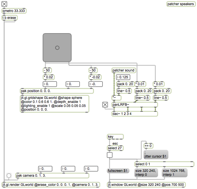
Example 26: Quadraphonic panning with mouse control and Open GL visualization
Example 27: Quadraphonic panning based on radial angle
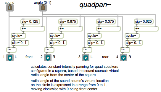
Example 28: Gain factors for quadraphonic panning based on radial angle
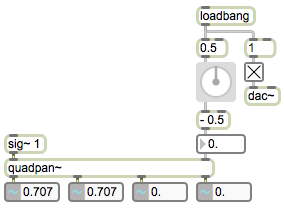
Example 29: Circular quadraphonic panning
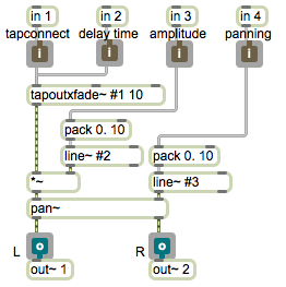
Example 30: Abstraction for delay with stereo panning
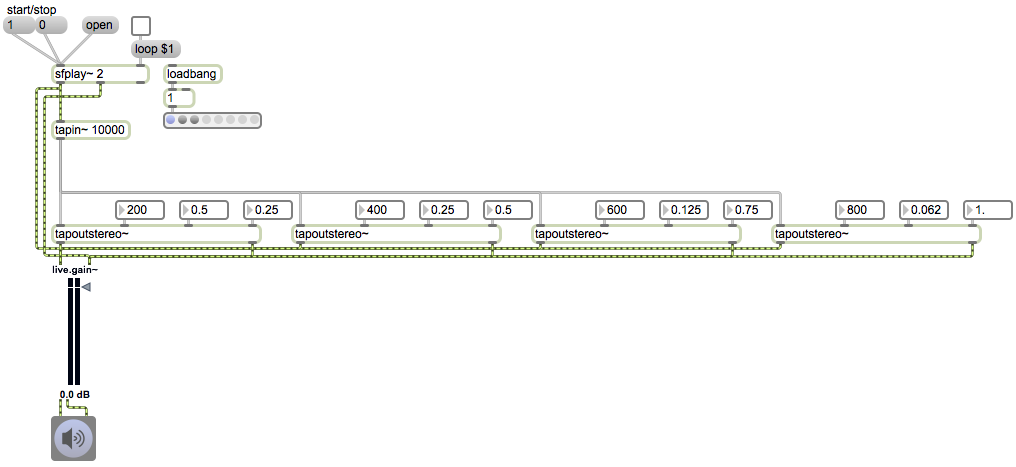
Example 31: Multiple delays with stereo panning
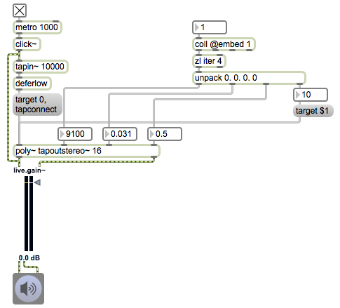
Example 32: Polyphonic panned delays with poly~
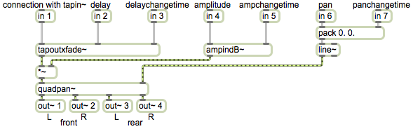
Example 33: Abstraction for delay with quadraphonic panning
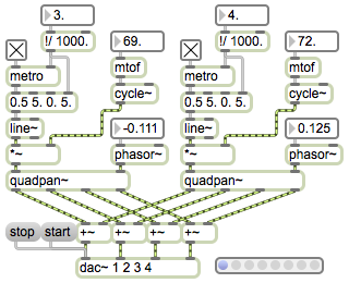
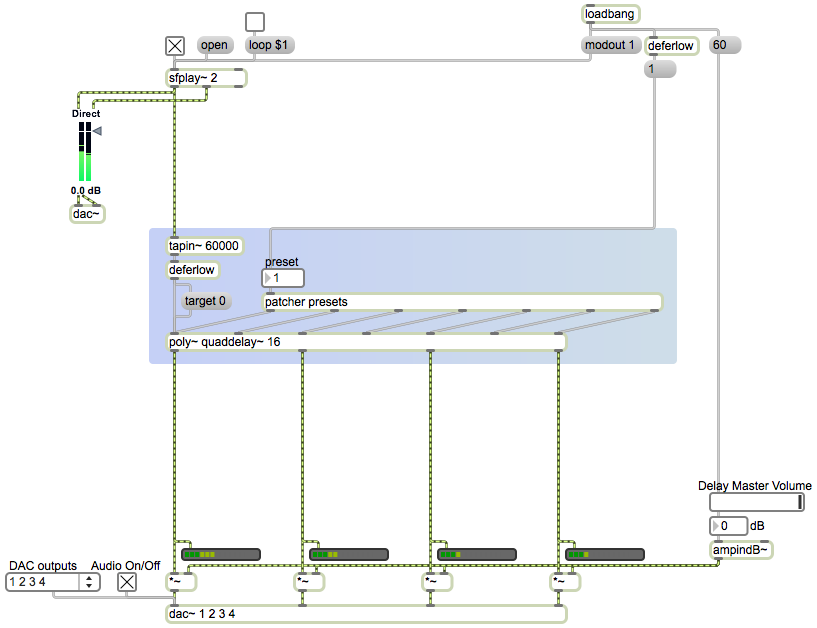
Example 34: Polyphonic quad-panned delays with poly~
This page was last modified May 5, 2012.
Christopher Dobrian
dobrian@uci.edu