Programming examples for the class
Music 215: Music Technology - Spring 2013
University of California, Irvine
This page contains examples and explanations of techniques of interactive arts programming using Max.
The examples were written for use by students in the Music Technology course at UCI, and are made available on the WWW for all interested Max/MSP/Jitter users and instructors. If you use the text or examples provided here, please give due credit to the author, Christopher Dobrian.
There are also some examples from the previous classes available on the Web: examples from spring 2012's Music Technology seminar, examples from 2012's Interactive Arts Programming class, examples from 2011's Music Technology class, examples from 2010's Interactive Arts Programming class, examples from 2009's class, examples from 2007's class, examples from 2006's class, examples from 2005's class, and MSP examples and Jitter examples from 2004's class.
While not specifically intended to teach Max programming, each chapter of Christopher Dobrian's algorithmic composition blog contains a Max program demonstrating the chapter's topic, many of which address fundamental concepts in programming algorithmic music and media composition.
You can find even more MSP examples on the professor's 2007 web page for Music 147: Computer Audio and Music Programming.
And you can find still more Max/MSP/Jitter examples from the Summer 2005 COSMOS course on "Computer Music and Computer Graphics".
Please note that all the examples from the years prior to 2009 are designed for versions of Max prior to Max 5. Therefore, when opened in Max 5 or 6 they may not appear quite as they were originally designed (and as they are depicted), and they may employ some techniques that seem antiquated or obsolete due to new features introduced in Max 5 or Max 6. However, they should all still work correctly.
[Each image below is linked to a file of JSON code containing the actual Max patch.
Right-click on an image to download the .maxpat file directly to disk, which you can then open in Max.]
Examples will be added after each class session.
Example 1: A useful subpatch for mixing and balancing two sounds
To mix two sounds together equally, you just add them together. If you know that both sounds will frequently be at or near full amplitude (peak amplitude at or near 1) then you probably want to multiply each sound by 0.5 after you add them together, to avoid clipping. However, if you want to mix two sounds unequally, with one sound having a higher gain than the other, a good way to accomplish that is to give one sound a gain between 0 and 1 and give the other sound a gain that's equal to 1 minus that amount. Thus, the sum of the two gain factors will always be 1, so the sum of the sounds will not clip. When sound A has a gain of 1, sound B will have a gain of 0, and vice versa. As one gain goes from 0 to 1, the gain of the other sound will go from 1 to 0, so you can use this method to create a smooth crossfade between two sounds.
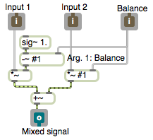
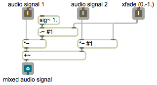
This example employs that mixing technique and implements it as a patch that can be used as an object inside another patch. It's handy for easily mixing and/or adjusting the balance of two audio signals. Save the patch as a file with a distinct and memorable name such as "mix~.maxpat" somewhere in the Max file search path. Then you can use it as a subpatch (also often called an "abstraction") in any other patch just by making an object named "mix~". The audio signals go into the left and middle inlets and the mix value from 0 to 1 goes into the right inlet. There are three ways to specify the balance: 1) as an argument typed into the object box, 2) as a float in the right inlet, or 3) as a signal in the right inlet. Using a signal to control mixing is the best choice if you intend to change the mix dynamically.
Whatever goes in the inlets of the mix~ object in the main patch comes out the corresponding inlet objects in the mix~ subpatch, and the mixed signal comes out the outlet. The sig~ object provides a constant signal in which every sample has the same value, in this case a constant value of 1. The argument #1 will be replaced by whatever is typed into the mix~ object box as an argument in the parent patch; if nothing is typed in, it will be 0, and if a signal is attached in the main patch then the signal value will be used. This allows the user to type in an argument to specify the initial balance value in one of the *~ objects, and the -~ object provides 1 minus that value to the other *~ object. That initial balance value can be replaced by sending in a float or a signal.
Example 2: Linear audio crossfade
This example uses the subpatch from the previous example, so it requires that you download the file mix~.maxpat and save the file, with that same name, somewhere in the Max file search path.
This example demonstrates the use of the line~ object to make a linear control signal, which is used to control the balance between two audio signals. (A "control signal" is a signal that's not intended to be heard directly, but which will affect some aspect of another signal, or perhaps will control some global parameter of several sounds.) The line~ object receives a destination value and a ramp time, and it then interpolates, sample-by-sample, from whatever its current value is, to ramp to the specified destination value in exactly the desired amount of time.
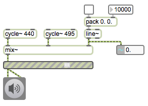
The mix~ object expects a control signal from 0 to 1 in its right inlet to specify the desired balance between the two audio signals in its left and middle inlets. When the control signal is 0, we hear only the first input sound; when the control signal is 1, we hear only the second input sound. Inside mix~, the two sounds are scaled appropriately according to the balance value in the right inlet, added together, and sent out the outlet. So to do a smooth linear crossfade between sound 1 and sound 2, it makes sense to send a linear control signal from 0 to 1 into the right inlet.
The two cycle~ objects provide constant full-amplitude tones (the pitches A and B), so they're good sound sources to allow us to hear the effect of the crossfade clearly. The toggle is used to initiate a crossfade from one sound to the other; it provides a 1 or a 0 as the destination value for the balance. First we need to supply a ramp time, in milliseconds, in the right inlet of the pack object. When the destination value comes from the toggle, it gets packed together with the ramp time as a two-item list, and passed to the left inlet of line~. Over the course of that specified time, line~ calculates the intermediate value for each sample that's needed in order to describe a straight linear progression toward the destination value.
The line~ object is thus a control signal generator, and importantly, it's an object that provides an interface between the Max scheduler (the normal world of Max in which individual messages occur at a specific instant in time) and the MSP signal chain (in which a continuous stream of audio samples are being calculated). A single message to line~ triggers a change in its output signal, a change which could take place over any desired amount of time. You can also think of line~ as a "smoother", allowing a signal parameter (such as amplitude, frequency, etc.) to change smoothly from one value to another.
Example 3: Using matrix~ for multi-channel audio amplitude control
This example shows how to control the amplitude of multiple signals with the matrix~ object, instead of with line~ and *~ objects. In effect, matrix~ has the linear interpolation and multiplication capabilities of those objects embedded within it.
The matrix~ object can be thought of as a mixer/router of audio signals. The arguments to matrix~ specify the number of audio inlets, the number of audio outlets (there's always one additional outlet on the right), and the initial gain for the connections of inlets to outlets. Each inlet is potentially connectable to each outlet with a unique gain setting; the gain of the connections is changed by sending messages in the left inlet.
The messages in the left inlet of matrix~ specify an inlet number (numbered starting from 0), an outlet number, a gain factor for scaling the amplitude of that connection, and a ramp time in milliseconds to arrive at that amplitude. You can send as many such messages as needed to establish all the desired connections.
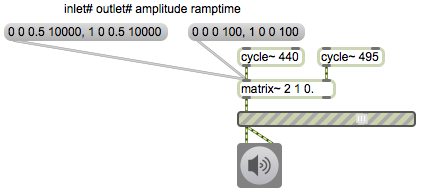
In this example we have a matrix~ with two inlets and one outlet. A full-amplitude sinusoidal audio wave is coming in each inlet, but we don't hear anything initially because the third argument of the matrix~ has set the initial gain of all connections to 0. When you click on the left message box, it sends two messages meaning, "Connect inlet 0 (the leftmost inlet) to outlet 0 (the leftmost outlet) with a gain factor of 0.5 getting there in 10 seconds, and also connect inlet 1 to outlet 0 with a gain of 0.5 getting there in 10 seconds as well." When matrix~ receives those two messages, it begins the linear interpolation of those connections to 0.5 gain over 10 seconds. (We chose a gain of 0.5 so that the sum of the signals would not exceed 1.) When you click on the message box on the right, it will set the gain of both of those connections to 0 in 100 milliseconds.
This method of sending a message for each possible connection may seem a bit cumbersome when you're controlling a matrix with many inputs and outputs, but in fact it's about the most efficient way to control a large matrix (a virtual patchbay) of possible connections. With some clever message management, you can control or automate a great many constantly-changing connections. You can re-route inlets to outlets as need be, and you can control the amplitude of all the connections.
For some slightly more elaborate examples of the use of matrix~, see the examples called Using matrix~ for audio routing and mixing and Mixing multiple audio processes.
Example 4: The function object
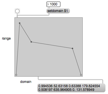
The function object assists you to make shapes composed of line segments. When you send a bang to the function, it sends out of its second outlet a list of destination value and ramp time pairs suitable for use as input to a line~ object. In that way, the shape shown in the function object serves as a function over time, the shape of which will be enacted by the signal coming out of the line~ object.
A two-dimensional graph like the one shown here shows the relationship between two variables, x and y, and is said to be a graph of "y as a function of x" or "y over x". That means that it shows how the y variable changes with each corresponding x value. In most musical situations, the x axis designates time (with x=0 designating a starting point in time) while y designates a value that changes over time according to a certain shape or curve. Since the x value (time) increases at a constant rate, the shape of the function shows us how y will change over time.
In math terminology, the minimum and maximum of the numbers on the x axis are said to determine the "domain" of the function, and the minimum and maximum of the numbers on the y axis determine the "range" of the function. By default, the domain of the function object is 0 to 1000 (since it's assumed that the domain will designate milliseconds), and the range is 0 to 1. But you can change the extent of the domain and the range with the messages setdomain and setrange. The minimum of the domain is always 0 in the function object, so you only need to provide the desired maximum with the setdomain message, as in setdomain 1000. For the range, you specify both the minimum and the maximum, as in setrange 0. 1.
Try changing the domain and the range, and then sending a bang to see how the resulting list changes. Notice that in this patch we use the pak object to combine the minimum and maximum values in a single setrange message. The pak object is used to combine several individual numbers together into a list, much like the pack object. The crucial difference between the two is that the pak object sends out a list any time it receives something in any inlet, whereas the pack object sends out a list only when it receives something in its leftmost inlet.
Example 5: Amplitude envelope with the function object
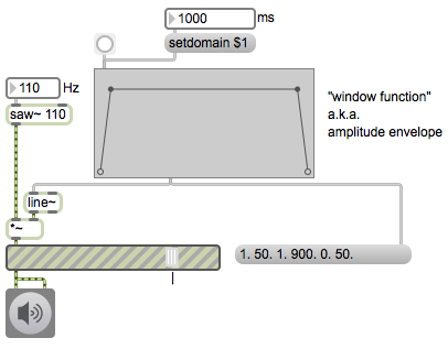
In MSP, each MSP object (each object that has signal input and/or output) is always producing signal as long as audio is turned on. For example, signal generators like cycle~ (sinusoidal wave generator) and saw~ (band-limited sawtooth wave generator) are always producing a full-amplitude wave. You control the amplitude of that wave with multiplication, using *~ or some other object that performs a multiplication internally (such as gain~). Multiplication by a value greater than 1 increases the amplitude (amplification), and multiplication by a value between 0 and 1 decreases the amplitude (attenuation). (Multiplication by a negative number has the same sort of effect, while also inverting the signal about the x axis.) Multiplication by 0 completely suppresses the signal (silence). In that last case, the signal generator is still working just as hard, producing its full amplitude signal, but the multiplication by 0 converts every sample to 0.
You can think of every individual sound as being surrounded by silence. You could imagine that, as in MSP, sound is always present, but during the silence its amplitude is 0 (the sound is being multiplied by 0), and when the sound is audible it is being multiplied by 1 or by some other nonzero number. Thus, the sound is audible only when its amplitude is being controlled by a nonzero value -- a conceptual "window" is opened on the sound allowing it through -- and the rest of the time it's being multiplied by 0 and the conceptual window is closed. This idea of a "window" -- a period of nonzero values surrounded by 0 before and after -- is an important concept in digital music and in digital signal processing. A sound that is off (0), then is instantaneously switched on (1), then is later instantaneously turned off again (0) has been windowed with a rectanglar-shaped function. More commonly in music software we use a window shape that is not exactly rectangular, such as a trapezoidal window with tapered ends, to avoid clicks.
This example demonstrates the use of a function object to create a trapezoidal window signal coming out of the line~ object to control the amplitude of a sawtooth oscillator. Each time function receives a bang, it sends out a list that says, "Go to 1 in 50 milliseconds, stay at 1 for 900 milliseconds, then go to 0 in 50 milliseconds." The changing values from line~ are used as the multiplier controlling the amplitude of the oscillator, opening a 1-second window on the sound.
The duration of that window can be changed simply by sending a setdomain message to function. Note that the duration of each segment of the function is time-scaled proportional to the domain specified, so the fade-in and fade-out tapered ends of the function, which are 50 milliseconds initially, would last only 5 milliseconds if the duration of the window were shortened to 100 ms, and would last 500 milliseconds if the total duration (the domain) were set to 10,000 ms.
Example 6: Interpolation with the function object
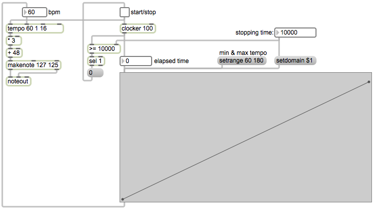
The function object can be used to create line segment functions that control a line~ object, and it can also be used as a lookup table. A number coming in its inlet will be treated as a point on the x axis, and whatever y axis value is shown on the line segment function at that point will be sent out the leftmost outlet. This example patch demonstrates that use of function.
The function object in this patch has been saved with its domain set at 10,000 and its range set from 60 to 180. Click on the toggle to see and hear what this patch does. When the toggle is turned on, it sends out the number 1, which turns on the clocker object, which in turn begins to report the time that has elapsed (starting at 0 at the moment it's turned on) at regular intervals specified by its argument (every 100 milliseconds in this case). The elapsed time is used to look up a tempo between 60 and 180 in the function object, and that tempo is sent to the tempo object to determine its (quarter note) beats per minute. The elapsed time value from the clocker is also used to check whether the stopping time has been reached, which initially is 10,000 milliseconds. Finally, the 1 from the toggle will be used to start the tempo object, which will have already received the correct tempo from the function. When clocker reaches 10,000, the >= object will send out the number 1, which will be detected by the sel 1 object, which will turn off the clocker and the tempo object. Thus, as the elapsed time progressed from 0 to 10,000 (or whatever you set as the stopping time), those increasing numbers read through the function that is in the lookup table, i.e., the line segment shape designating musical tempo that is in the function object.
The upper left portion of the patch is a very simple note generator. The tempo object is set to output numbers designating sixteenth notes at whatever quarter-note tempo it receives. The first argument is the initial tempo, and the next two arguments are the numerator and denominator of a fraction saying what kind of note value it should use as its output rate, in this case 1/16 notes. The tempo object will send out the numbers 0 to 15 showing which 16th note it's on within a standard 4/4 meter. At the downbeat of each 4/4 measure, it wraps back around to 0 and repeats. Those numbers from the tempo object are multiplied by 3, thus counting by threes from 0 to 45, and then added to 48 so that it's now counting by threes from 48 to 93. Those numbers 48, 51, 54, 57,...93 are used as pitch values in the makenote object, which combines them with a velocity value of 127 and sends 125-ms-long MIDI notes to the noteout object. The result is a four-octave arpeggiation of a C diminished seventh chord.
Try changing the domain of the function to play phrases of different durations. Try clicking in the function to create new points, making whatever shape of tempo changes you'd like to try. (You can shift-click on points to delete them.)
Example 7: Line segment function as a musical motive
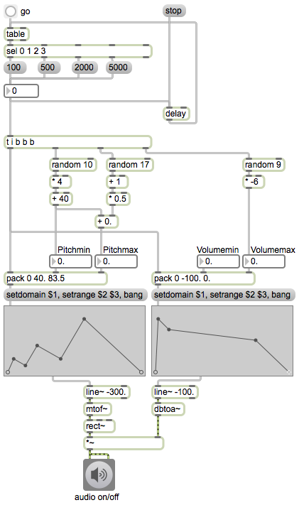
This example is from my Algorithmic Composition blog, and is explained there.
This patch uses the table object to calculate a probablility distribution to make the short notes occur much more often than the long notes. We'll discuss that in a future class, but feel free to read about it now if you're interested.
Example 8: Basic linear mapping
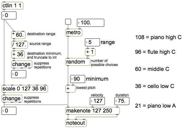
The most direct way to convert one range of numbers into a different range of numbers is a process called linear mapping. For each number in a source (input) range, find the corresponding number in a destination (output) range. The process is to multiply the input value by the size of the destination range (destination maximum minus destination minimum) divided by the source range (source maximum minus source minimum), then add the destination minimum to that. In short, the conversion operation involves scaling and offsetting: one multiplication and one addition.
The scale object does this for you. In this example we want to convert the incoming MIDI control data from the mod wheel of a synthesizer, ranging from 0 to 127, into a usable pitch range from 36 (cello low C) to 96 (flute high C). The patch demonstrates the use of the scale object, and also demonstrates that you can obtain the same result with basic arithmetic objects. Notice that, because there are no arguments with a decimal point in the scale object, the result is sent out as an integer. For a floating point result, at least one argument of scale must be a float. The patch emulates that behavior by using an integer addition in the + object, which truncates any fractional portion of the number coming from the / object. Because the input range is greater than the output range, and we're dealing only with whole numbers, there will be some duplication of numbers in the output, so we filter out repetitions with the change object.
A similar process can be used to get any range of random numbers we want. First we establish a range of random numbers (for example, if we send 6 into the right inlet of the random object, the range of its output will be from 0 to 5), then we offset it by whatever value we want to be the minimum result.
Example 9: Table lookup
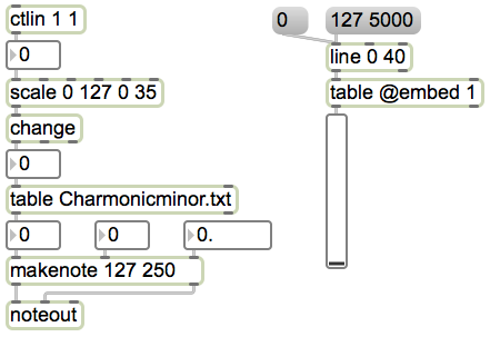
The table object is what's commonly called a "lookup table" or an "array". You can store an ordered array of numbers, and then look up those numbers by referring to their "index" number (also sometimes called the "address") in the array. In table, the index numbers start from 0, and each location in the array can hold an integer. In the table's Inspector, you can set it to save its contents as part of the patch, so that the stored numbers will always be there the next time you open the patch. When table receives an index number in its left inlet, it sends out the number that is stored at that index location.
In this patch, we use a table to store all the MIDI pitch numbers of the C harmonic minor scale from 36 to 96, and we use another table to store a shape -- a drawn curve. (You can double click on the table objects to see their contents displayed graphically.)
To make a lookup table filled with a specific ordered set of integers, the table object is the best choice, and one way to fill it is to read in a text file that begins with the word "table" followed by a space separated list of the desired numbers. This example patch requires that you download the text file Charmonicminor.txt and save it with the correct name somewhere in the Max file search path.
You can use a lookup table to describe some curve or shape that's not easily calculated mathematically, anything from a harmonic minor scale to a curve you draw freehand. The table object on the right has had a curve drawn into its graphic window, and its embed attribute has been set on, which has the same effect as choosing "Save Data With Patcher" in the object's Inspector.
Example 10: Refer to a lookup table remotely
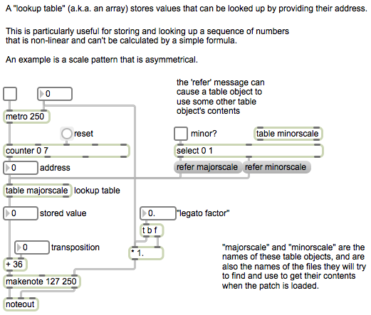
You can temporarily change the name and contents of a table object with the refer message, referring to the contents of another named table. In this patch we use a toggle to switch between a major scale and a minor scale, triggering the necessary refer messages. Once we refer the table named "majorscale" to the table named "minorscale", the table named "majorscale" actually adopts the name and the contents of the table named "minorscale" as if it were its own (although the name that was typed in as an argument does not change). The major scale content does not disappear entirely, however. It's still in Max's memory, stored as a table with the name "majorscale", so the table object can be restored to its original name and contents by the message refer majorscale.
The name that's typed in as an argument also serves as the name of a text file that the table object will try to read when the patch is opened. If no such file is found, the table will be empty (all it values will be set to 0) or it will use the saved data if its embed attribute is set (its "Save Data With Patcher option was checked). In this example patch, the data of the two scales is embedded in the patcher file, but can also be stored in separate files named majorscale and minorscale.
The basic scale pattern of pitch classes then needs to be transposed my some number to put it in the desired key and register. The patch also includes a "legato factor" applied to the duration of the notes. The time between note onsets, also known as the "inter-onset interval" or "IOI", is determined by the metro interval. That value is then multiplied by the legato factor to determine the actual duration, from attack to release, of each note. In this way, the duration of the notes is dependent on, but not identical to, the IOIs. A legato factor greater than 1 creates note overlap, while a legato factor less than 1 creates a détaché or staccato effect.
Example 11: Sequential or random access of a lookup table
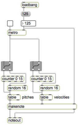
One of the nice features of an array is that you can store data in a particular order, then recall it in that order simply by incrementing an index counter. Or you can access the data randomly, which still restricts your outcome to members of that data set but ignores the original order.
This patch demonstrates that with a 16-value array of pitches and another 16-value array of velocities. When you turn on the metro, originally both arrays are read in order, and each contains a distinctive pattern. Try clicking on the gGate objects to switch one or both of them over to random access of the table, to hear the effect of randomizing one musical parameter or both.
Example 12: Random voicings of a pitch class set
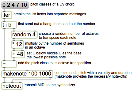
A chord can be described as a pitch class set. For example, a C dominant ninth chord is the pitch class set {0,2,4,7,10}. Depending on the octave transposition of each of those five pitch classes, many voicings of the chord are possible. This patch take applies a transposition of four, five, six, or seven octaves to each of the five pitch classes to create a random voicing of the chord.
First the list is broken up into five individual messages by the iter object. Then for each of those numbers, the trigger object (t) first sends out a bang to choose a transposition of 48, 60, 72, or 84, then sends out the pitch class to be added to that transposition. The five pitches are played practically simultaneously with a velocity of 100, and 1 second later makenote sends out a note-off for all five notes.
Example 13: Look up chords in an array
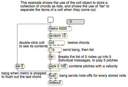
The coll object allows one to store an indexed collection of messages of any type. In this example, each stored message is a list of five numbers that will be used as pitches of a chord. (Double-click on the coll to view its contents.) The chords are chosen at random, but they have been composed such that they all have a valid function in C minor, and because they are all five-note jazz chords voiced in a similar manner and range, stylistically any one of the twelve chords sounds reasonable following any other.
The iter object breaks up each list into five separate int messages, each of which is packed together with the number 100 as a two-item list, and that list is passed to noteout as pitch and velocity information.
This patch demonstrates an effective way to provide note-off messages for MIDI notes. Pitch and velocity pairs can be passed through the flush object, and flush will memorize all pairs that are note-ons -- that is, pairs in which the velocity is nonzero; then, when flush receives a bang, it outputs note-offs for each note-on that it has in memory that has not yet been followed by a note-off. In this patch, each time a list comes out of the coll, it triggers a bang to turn off the held notes of the previous chord before playing the next chord.
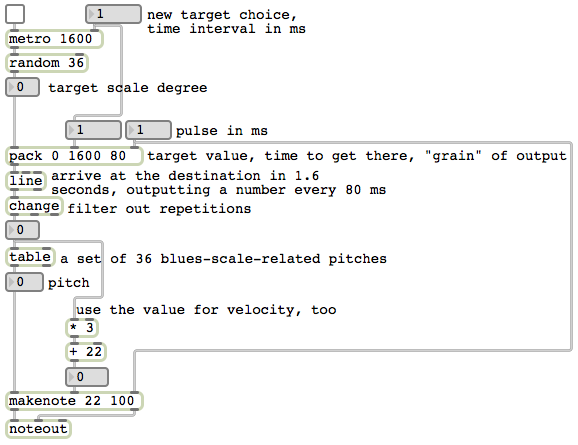
Example 14: Automated blues "improviser"
Example 15: Random semitone trills

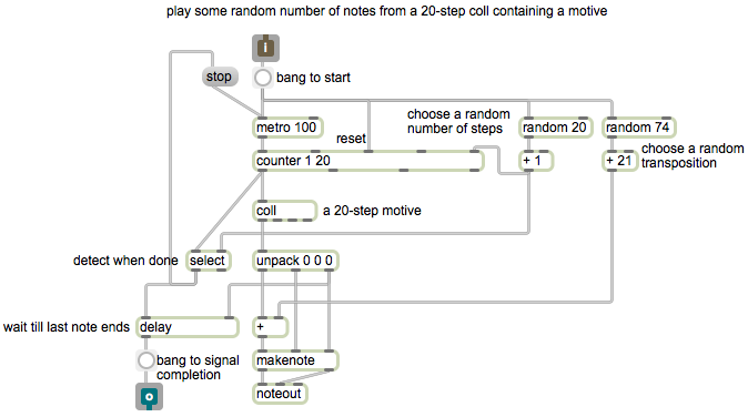
Example 16: Motivic "improviser"
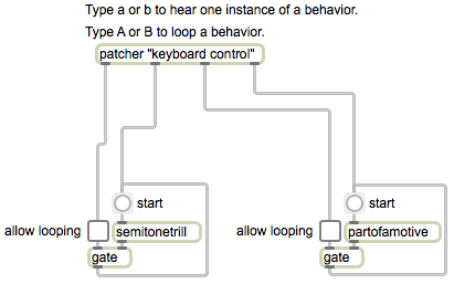
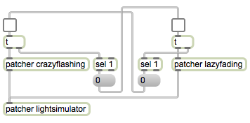
Example 17: Choose from among multiple processes
Example 18: Automated minimal composer
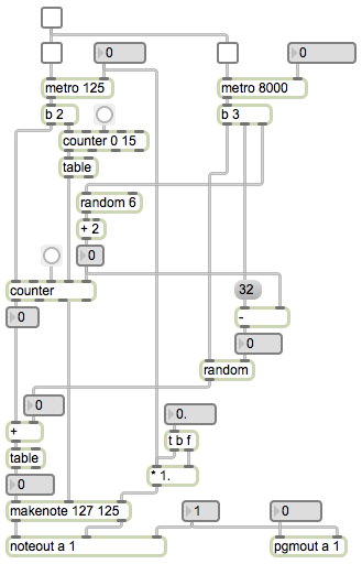
This patch composes a melody in Minimal style, playing periodically-varying diatonic melodic loops of different lengths. A 16-stage sequence of velocity values is stored in one table, and a 32-stage sequence of pitch values is stored in another table. The velocity values are carefully chosen to produce a pattern that essentially reinforces a metric interpretation of sixteenth notes in 4/4 meter, with a strongly accented downbeat and moderately accented beats 2, 3, and 4, but with a few other accents that are slightly at odds with the 4/4 interpretation, giving a sense of syncopation. The pitch values are composed using only six different pitch classes (Ab, Bb, C, Db, Eb, F), spanning a two-and-a-half-octave range and with frequent small leaps.
The velocity values are always read in order, so that the impression of a syncopated 4/4 meter is maintained inflexibly. However, the melody is composed by looping different short segments of 3 to 8 values from the pitch table, changing every four measures. The pitch pattern of the melody therefore is frequently implying a different periodicity than the velocities, adding another layer of rhythmic complexity. And because of the frequent small melodic leaps in the pitch patterns combined with the rapid rate of performance, the listener tends to cognitively stream imagined counterpoint within the melody. The periodic changes in pitch pattern and register, combined with the rhythmic variety, keep the music engaging for quite a while.
Example 19: Automated countermelody improviser
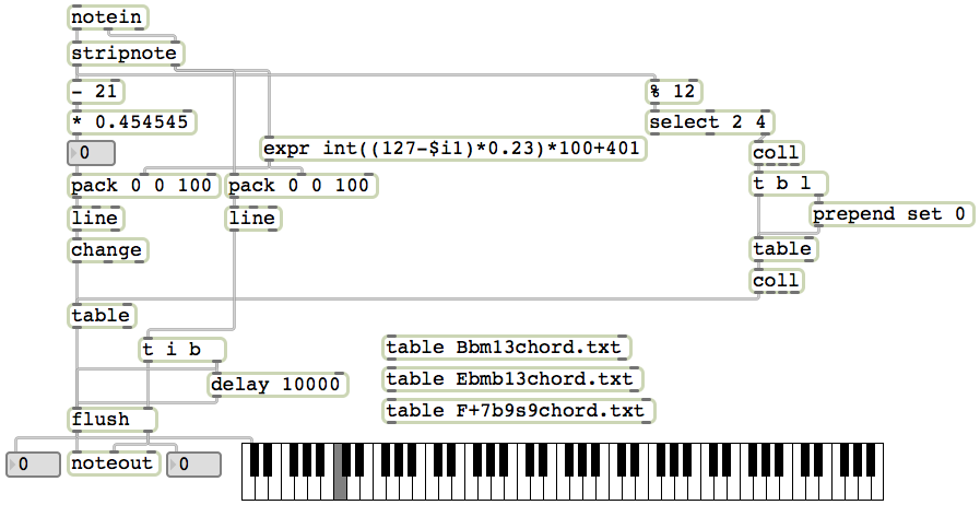
This patch provides an example of simple interactive improvising program that plays a melody influenced by the notes played by a live performer. Based on the most recently received MIDI note, the program chooses a scale to use for its melody, and moves melodically in a straight line toward the pitch and velocity most recently received. The program has only one use of randomness, to make a probabilistic decision. It has a small musical knowledgebase of three scales, and a set of probabilities determining which scale is more appropriate for use at any time.
When a MIDI note comes into the program via the notein object, we use a stripnote object to suppress the note-off messages, so we're only paying attention to the note-ons. The velocity is used to affect how quickly the program will move from its own most recently played note to the note it has most recently received. Some math in an expr object is used to convert the note-on velocity value into a ramp time value for the line objects. The pitch value is first used to determine what scale the program should use for its melody, then it is used to determine a destination point for its own melody that is near the received note.
Here's how the note choices are made. There are three table objects containing three different musical scales. I call them scales, but one might equally well call them chords. They're based on six-note pitch class sets, each one having a particular harmonic implication. The names of the table objects indicate the chord type, using jazz terminology, Bbm13, Ebm9b13, and F+7b9#9. Thus, the program is biased toward the key of Bb minor. The upper coll object contains probabilities for choosing each of the three scales. (Double-click on the coll object to see its contents.) Using a % object we derive the pitch class of the incoming MIDI note, using the sel object we filter out the notes D and E (since those don't seem to imply any particular one of the three possible scales, we just ignore them and continue using whatever scale we have been using), then use the pitch class to select a set of probabilities. Those probabilities are temporarily stored in a small table.
The table object has a feature that allows it to act as a probability table. When table receives a bang, it treats its values as relative probabilities, and based on those probabilities it chooses to send out out an index number (not the value itself). Thus, index numbers containing higher values tend to be sent out more often, with a likelihood proportional to the value it contains. We use that feature of table, along with the probabilities received from the first coll, to determine which index to send out -- 0, 1, or 2. That index is used to choose a message from the second coll, which tells another table object which scale table it should refer to. As soon as that's done, a destination value is calculated and sent to a line object, which begins reading through the table, playing notes of the chosen scale.
Each velocity value the program plays triggers a bang to the flush object to turn off the previously played note. It also uses the delay object to prepare a final bang to be sent if no new note is played for ten seconds. The contents of the coll and table objects are all embedded in the patch (that is, their embed attribute is set to 1, so they will "Save Data with Patcher"). Since the table objects will also use that name to try to find a file to read in, you might want to include these three files just to avoid unwanted "can't find file" messages: Bbm13chord.txt, Ebmb13chord.txt, and F+7b9s9chord.txt.
Example 20: Amplitude and decibels
This example is a duplicate of an example from a previous class, and is described on the Examples page there.
Example 21: Frequency and pitch
Example 22: Time interval and rate
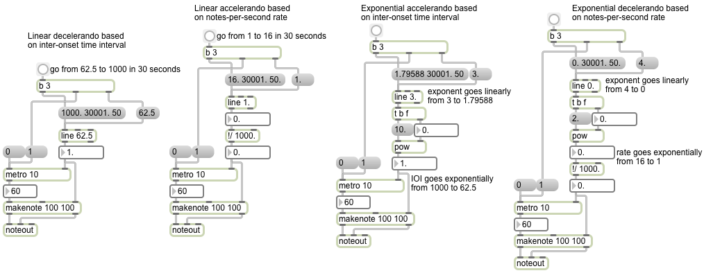
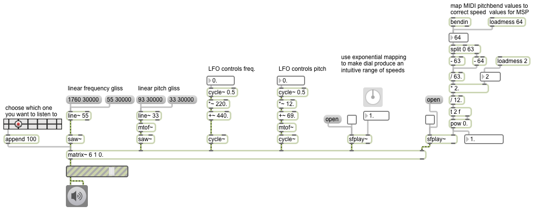
This patch provides examples that compare linear rate changes to exponential rate changes. As with pitch and loudness, our sense of change in the rate of events is based on the ratio of tempos rather than the (subtractive) difference between tempos. In these examples, the rate changes by a factor of 16, from 1 event per second to 16 events per second, or vice versa. In the first example, we use a linear change of time interval for a metro, to go gradually from 62.5 milliseconds to 1000 milliseconds, which is to say from 16 notes per second to 1 note per second. By changing the time interval linearly, we get a larger change in the notes-per-second rate initially than we do later in the accelerando, which means that most of the change in perceived tempo takes place in the earliest part of the thirty seconds. In the second example, by contrast, we use line to effect a linear change in the notes-per-second rate (tempo), which actually causes an increasing rate of change in the time interval being provided to metro, but results in an accelerando that seems (and in fact is) more constant over the course of the thirty seconds, and is thus more musically useful. In the two examples on the left the change, be it of time interval or rate, is linear. In the two examples on the right, the output of line objects is used as the exponent in a pow object, thus converting the linear rate change into an exponential one. This yields, in most cases, a smoother and more "musical" sense of accelerando or decelerando. Exactly which method of change you choose to use depends on which most closely corresponds to the musical effect you're trying to achieve.
Example 23: Using the timepoint object to specify exact points in musical time
This example is a duplicate of an example from a previous class, and is described on the Examples page there.
Example 24: Convert between musical time and clock time
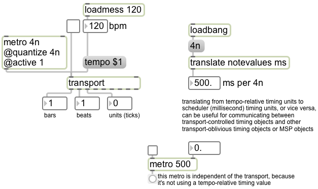
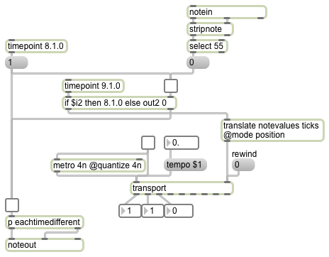
The translate object performs conversions from one kind of time unit to any other, and is particularly useful when you need to convert from a tempo-relative time unit to a clock time unit (e.g., convert note values to milliseconds) or vice versa. In this example, try changing the bpm tempo of the transport, and you'll see that the translate object sends out updated information whenever the tempo changes.
A very similar example from a previous class gives additional explanation.
Example 25: Bass drum player with swing
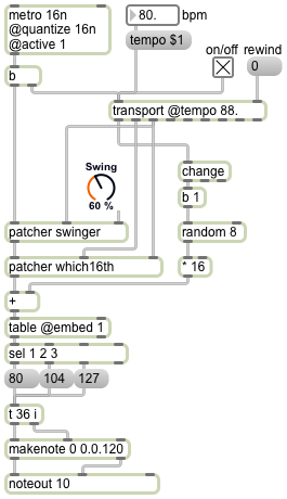
This patch uses the transport object to control an algorithmic performer of kick drum patterns. When the transport is turned on, the metro also turns on because its active attribute is set on. The metro sends a bang on every 16th note. Those bangs are first used to trigger information from the transport itself, and then to look up in a table of patterns to see whether or not to play a bass drum note. Along the way, the bangs from the metro pass through a subpatch that applies a certain amount of delay--equal to some proportion of a 16th note--to every other 16th note, giving a variable amount of "swing" feel to the drum patterns.
For each bang of the metro, we get information from the transport: the bar number, the beat number, and the number of units (ticks) within the beat. On the right part of the patch, you can see that we use the change object to filter out repetitions of bar number, so we will only pass on the bar number when it changes, which is to say, on the downbeat of each bar. We use that downbeat indicator to choose a random number from 0 to 7, and multiply that by 16 so that we get the numbers 0, 16, 32, ... 112. That result gets stored in a + object. We'll see what it's used for in just a minute.
For now, let's ignore the patcher swinger object. We'll come back to that. Let's imagine that the bang from the metro is just going directly to the patcher which16th. The metro sends a bang on every 16th note, and the patcher which16th subpatch will tell us which 16th note of the measure is occurring, using numbers 0 to 15. (Side note: you could also use a counter 0 15 object to generate that information, but if the transport time were to be changed in some other patch, the counter could get out of sync with the downbeat, and would be providing incorrect information.) Double-click on the patcher which16th object to see its contents. Since there are 480 divisions per quarter note by default, and the metro is quantized to occur only on 16th notes, the units coming in the right inlet will always be 0, 120, 240 or 360. So we divide by 120 to get which 16th note of the beat it is -- 0, 1, 2, or 3. The beats coming in the middle inlet are numbered 1 to 4, so we subtract 1 and multiply by 4 to convert that to a number of 16th notes, add it to the 16th note offset from the units, and store the result in the right inlet of an i object. That's the 16th note index within the measure, numbered from 0 to 15. Then, when the bang from the metro comes in an instant later, it will send out the correct 16th note index.
We use that 16th note index to look up information in the table object. But before it gets to the table, it passes through the + object where we previously -- on the downbeat of each measure -- stored some offset 0, 16, 32, ...112. That means that for each measure, we will be looking up some different range of sixteen values in the table: 0-15, 16-31, 32-47, etc. up to 112-127. Double-click on the table object to see its contents. It stores 128 values ranging from 0 to 3. A table of 0s and 1s is useful for storing patterns of on/off information; in this case I decided to use numbers 0 to 3 so that the table could store four gradations: off, soft, medium, and hard. Every group of 16 values in the table is a unique composed rhythmic pattern of notes suitable as a kick drum rhythm in 4/4 time. Using the information derived from the transport, we read through a group of 16 articulation values to get one of 8 possible rhythmic patterns. The output of the table will always be numbers 0 to 3, which we use to trigger velocity values: 80, 104, 127, or no action (for 0). Those velocity values are passed to a noteout object that's set to transmit on MIDI channel 10 -- the channel designated for drums in the General MIDI specification -- and then a pitch value of 36 -- designated to mean kick drum in the GM specs -- is sent to noteout to trigger the note.
Now let's take a look at the patcher swinger subpatch. As you know, in various styles of jazz and popular music, 16th notes are played unevenly, with the duration of the first of each pair of 16ths being slightly longer than the second. You might just as well say that the onset time of the second of each pair of 16th notes is delayed slightly. This practice is known as "swing". Scientific musicologists who have studied the performance of music that involves swing have found that the amount of swing varies from one style of music to another, and is also dependent on the tempo of the music. So, rather than try to quantify swing as some particular rhythmic unit, such as a triplet 8th note, it may make more sense in computer music to quantify swing as some percentage of a beat, or of a half beat. That's how we do it in this patch. If you figure that normally an unswung 16th note is 50% of an 8th note (120 ticks for a 16th, and 240 for an 8th), then a swung 16th note might range from 50% (no swing) to 75% (extreme swing equal to a dotted 16th note) of an 8th note. So to specify how much swing we want, I provide the user with a live.dial object that has a range from 50 to 75 and its units displayed with a % sign. Regardless of the range of the live.dial or how its units are displayed, however, its right outlet will always send a float value from 0 to 1 based on the dial position. Now double-click on the patcher swinger object to see its contents.
Inside the patcher swinger subpatch, the 0-to-1 value from the live.dial gets multiplied by 60 to produce some number from 0 to 60. The "ticks" value from the transport, which will always be 0, 120, 240, or 360 in this case, gets divided by 120 to convert those numbers to 0, 1, 2, or 3. We then use a bitwise operator & 1 to look just at the least significant bit of that number (the 1s place of its binary representation) to see if the number is odd or not. If the number is odd, the & 1 object will send out a 1; if not, it will send out a 0. That gets multiplied by the number from 0 to 60 we got from the right inlet, gets packed together with the word "ticks", and is stored in the right inlet of the delay object as a tempo-relative time value. It's the number of ticks we want to delay each 16th note: 0 delay for even numbered 16ths and some amount of delay for the odd numbered 16ths. (Remember, we're indexing the 16th notes of the measure starting from 0.) 0 ticks is no delay, and 60 ticks is a 32nd note's worth of delay. So each bang that comes in the left inlet gets delayed by some amount, depending on whether it's the first or second of a pair of 16ths, and based on the amount (percentage) of swing specified in the main patch.
I worked with only the kick drum in this example, so that the patch would not become too complicated, but one could duplicate this procedure for all of the other instruments of the drum kit, with unique patterns appropriate to each instrument, to get a full constantly-varying automated drum performance.
Note that this patch requires virtually no modification to work as a MIDI plug-in in Ableton Live. One can copy and paste this patch into Max for Live, add the "Swing" live.dial to the Presentation, move it to the visible area of the Presentation (the upper left corner), and set the patcher to "Open in Presentation" in the Patcher Inspector. The control messages to the transport object would become superfluous because the Live transport would be in charge, but the bang messages to the transport object from the metro will still report the correct time so that the patch will work as it should. The swing function will have the same effect, and will be independent of any "Groove" setting the Live track might have.
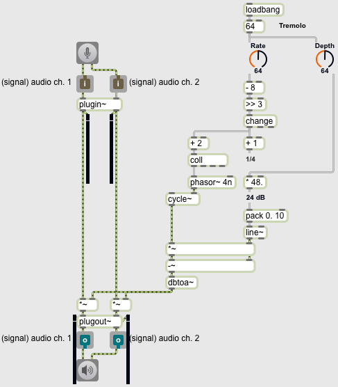
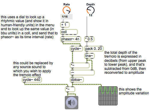
Example 26: Tremolo effect in Max for Live
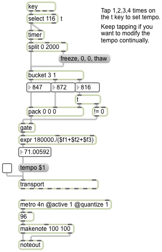
, Example 27: Tap to teach tempo to Max
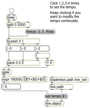
Example 28: Tap tempo utility in Max for Live
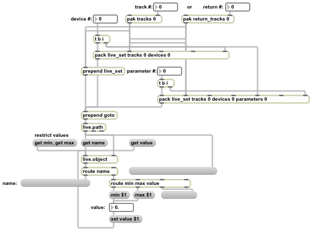
Example 29: Changing Live parameters with the Live API
Example 30: Live API via JavaScript
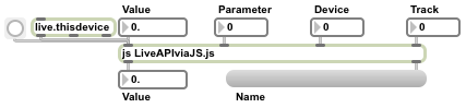
You can program the Live API in JavaScript if you prefer using a text-based procedural language. This Max patch demonstrates how to do that. For this demo patch to work, you will need to download the JavaScript file LiveAPIviaJS.js into the folder where you plan to save your Max for Live device, then download this patch and save it in the same folder as the JavaScript file (otherwise the patch will not find the .js file and the js object will not be created with the correct number of inlets and outlets), and then finally open the patch and copy and paste it into a Max for Live window.
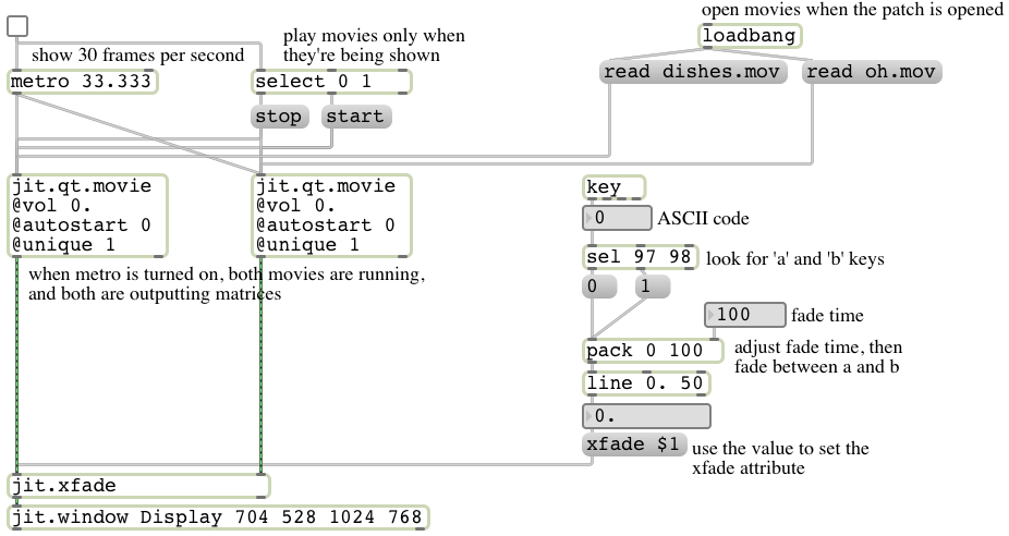
Example 31: A-B video crossfade
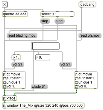
Example 32: Crossfade video and audio
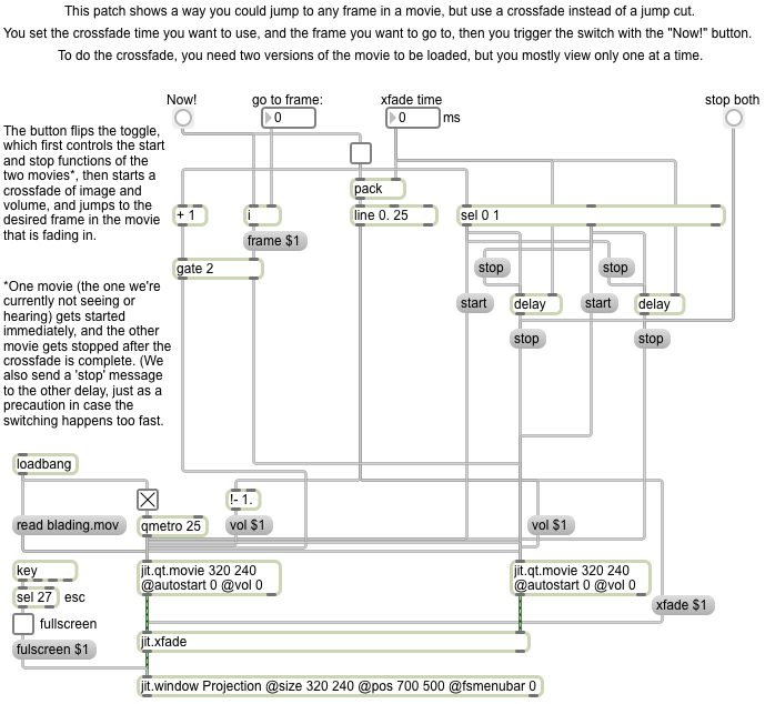
Example 33: Crossfade to new location in a video
Example 34: Create a sphere in OpenGL
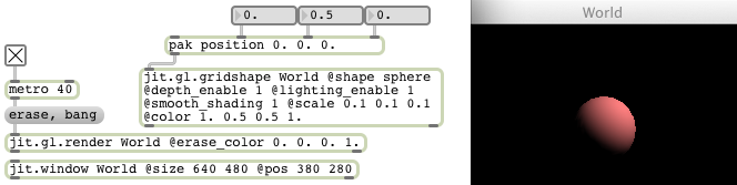
This example shows how to create and render a 3D shape in OpenGL. You can read about the meaning of some of the different attributes in Jitter Tutorial 33: Polygon Modes, Colors, and Blending and in the Max reference manual listing of common attributes and messages of Jitter GL objects.
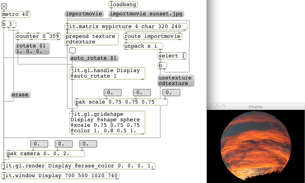
Example 35: Apply a texture to a shape in OpenGL
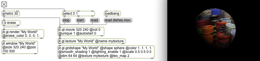
Example 36: Display a video on a shape in OpenGL
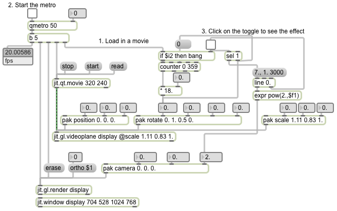
Example 37: Display a video on a plane in OpenGL
Example 38: Alphablend a videoplane in OpenGL
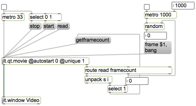
Example 39: Random frames of a video
Example 40: Simulation of MIDI lighting control
Example 41: Chaos algorithm for choosing pitches
.png)
Example 42: Sync tremolo to transport units
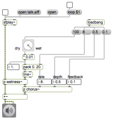
Example 43: A basic chorus effect
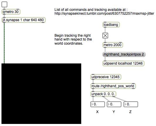
Example 44: Body tracking with Kinect and Synapse
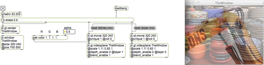
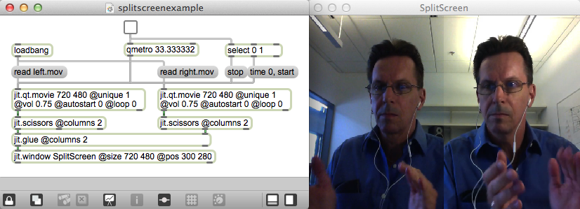
Example 45: Split screen video
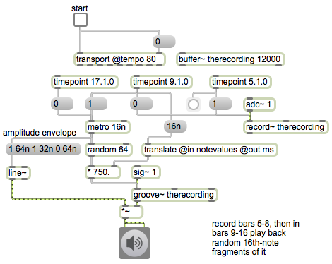
Example 46: Record and fragment audio in rhythmic units
Example 47: Testing for a range of numbers
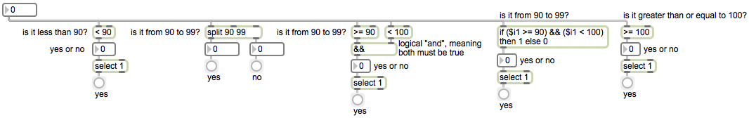
If you want to detect when a number has occurred that fits within a particular range, you'll want to use "logical operators" to test conditions such as "is less than", "is less than or equal to" or "is greater than this and less than that". Most logical operators send out the number 1 (meaning "true") if the condition is met, and 0 otherwise. The split object sends out its left outlet all input numbers that fall within a specified minimum and maximum, and sends the rest of its input numbers out the right outlet. The "and" operator && sends out a 1 if both of its inputs are true (non-zero), and 0 otherwise.
Example 48: Test movie timing to make editing decisions
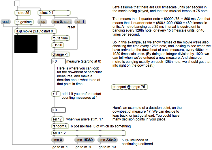
You can use the gettime message to ask jit.qt.movie for a report of its video's current time location (in QuickTime time units). The report comes out of the right outlet of jit.qt.movie as the word 'time' followed by the current time. If you send the gettime message at regular reliable intervals of time, you can use the resulting time number to test for a particular time (or range of times), and thus can take a particular action in your program at the desired time in a movie.
This can be useful for realtime editing of the movie itself, using the current time location to decide to leap to another location in the movie. In this case, we're assuming that we already know the timescale of the movie, and that we're synchronizing it with some music with a tempo of 75 beats per minute. So with a little arithmetic, we can figure out the relationship between milliseconds, QuickTime time units, and metric units of the music. In this example, we query (ask for and get) the movie's time every 25 milliseconds, which is every 1/40 of a second, which is 15 QuickTime time units at the timescale of 600, which is every 128th note in the music. And we can calculate that there are 480 time units per beat, and thus 1920 time units in a 4/4 measure of music. We do an integer division by 1920 to convert time units into measures, and thus can detect the downbeat of each measure.
In this example, when we get to the downbeat of measure 17 (i.e., after 16 measures have elapsed), we make a probabilistic decision. Should we go ahead, or should we jump back to a previous place in the movie? The example shows one model for weighted decision making; this model is useful if you have a really small set of choices and really simple probabilities. Here, three choices each have a 1/6 probability of occurring, and a fourth choice (to proceed ahead) has a 3/6 probability of occurring because 3 of the 6 possible random numbers do nothing.
Example 49: Granulation of a recorded sound
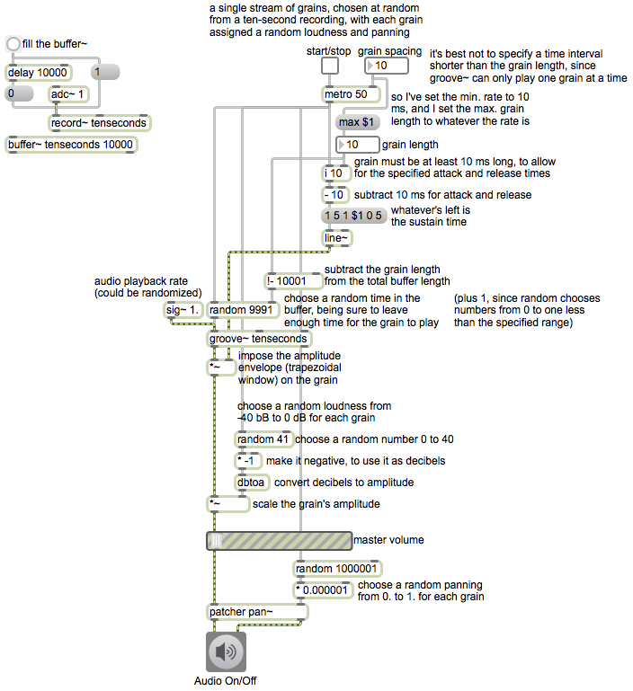
In classic granular synthesis, grains are very short windowed segments of sound, normally from 5 ms to 100 ms in length. A stream of sound grains be spaced at exactly the same time interval as the grain length, or at some greater interval of time. The spacing can even be randomized (some random time interval greater than or equal to the grain length). A single stream of grains is all you can do with a single groove~ object.
Although it's not demonstrated here, you could have a multiplicity of such streams going with multiple groove~ objects, or with multiple instances in a poly~ object, which would result in some overlapping of grains, making a "cloud" of grains, and if it's a dense enough cloud it starts to sound like one continuous sound.
This is an example patch that creates one steady stream of grains randomly chosen from a 10-second recording. You can set the grain length and the grain spacing to whatever timings you want. Here we use a 5 ms attack time and a 5 ms release time, so the minimum grain length in our case is 10 ms. Therefore, we limit the minimum grain spacing to 10 ms, too. (The number box setting the time interval for the metro object has had its minimum value set to 10 in the Inspector.) Each grain starts at a randomly-chosen start time in a 10-second buffer~. Each grain is also assigned a random loudness and a random panning. To make grains that are more like notes than grains, you can make grain lengths/spacings that are greater than 100 ms.
Example 50: Rhythmic automated panning
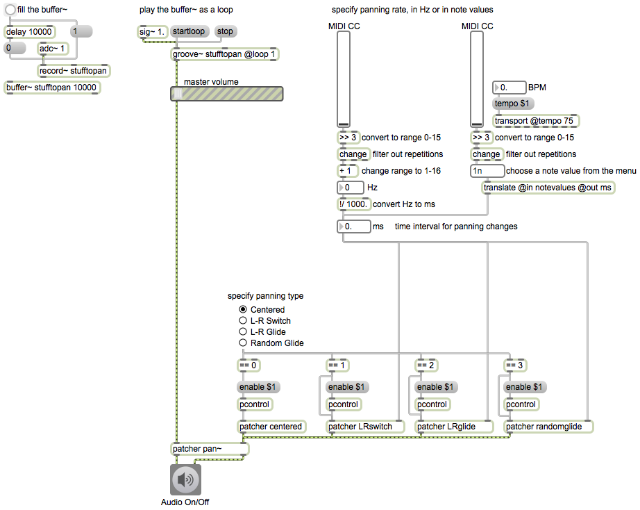
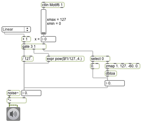
This example allows a choice of four different modes of intensity panning, and two ways to specify the rate of panning change. The choice of four possible pannings is: static centered, left-to-right sudden switching, left-to-right gradual gliding, and random gliding. The rate of change can be controlled by sliders, either in Hertz (changes per second) or note values (based on the current transport tempo).
A few objects and techniques here bear some explanation. The bit-shift operator >> shifts the binary form of an integer some number of bits to the right, which is equivalent to dividing by a power of 2. So shifting an integer 3 bits to the right is equivalent to an integer division by 8 (with the remainder being discarded). Why not just use a / 8 object? No reason (although it's perhaps a little more computationally efficient). It's just a nerdy way to scale down a range of numbers, by focusing only on the most significant bits of its binary form. The radiogroup object allows you to create a related set of mutually exclusive buttons, providing the user a choice of one (and only one) of several options. It sends out the index number of the selected button (counting up from 0).
The pcontrol object allows certain types of automated control of a subpatch or abstraction. One thing you can do is totally disable the MIDI and audio functions of a subpatch or abstraction, with the message enable 0 (and enable 1 to re-enable it). Inside those patcher objects that are getting enabled/disabled by the radiogroup, the audio chain of each one ends with a pass~ object. The pass~ object normally passes audio signals through unchanged, but it sends out a constant signal value of 0 whenever its patcher is disabled. This is crucial so that the subpatch doesn't get stuck sending out a constant non-zero signal when it's disabled. The fact that all the subpatches send out 0 when they're disabled means that they don't get in the way of the one subpatch that is enabled, when the signals all are added together in the right inlet of the patcher pan~ object.
Example 51: Abstraction for mixing or crossfading two audio signals
This patch is functionally identical to the mix~ abstraction in Example 1; you can read its explanation there. It's repeated here in order to begin a series of examples regarding "initialization": setting up the initial state of your program the way you want it. This patch demonstrates the use of a # argument in an object box to designate a value that can be specified in the parent patch when this patch is used as an abstraction (an object in some other patch). When this patch is used as an object in another patch by typing its filename into an object box, whatever is typed in as the first argument in that object box will be used in place of the #1, wherever it appears in this patch. (Subsequent arguments in the parent patch could be accessed with #2, #3, etc.) If nothing is typed in as an argument in the parent patch, the # arguments will be replaced by the integer value 0.
In this example, the #1 argument means that the initial crossfade value (to specify the balance between the audio signals coming in the first two inlets) can be typed into the object box in the parent patch. Notice that if the user does not type in any argument, the default behavior of this patch will be to send out only the audio signal of the left inlet, because the crossfade value will be 0 by default, resulting in a multiplier of 1 for audio signal 1 and a multiplier of 0 for audio signal 2.
[You can read a thorough explanation of the # argument in an excerpt from the Max 4 manual regarding the changeable arguments $ and #.]
An important thing to notice in this abstraction is that it has been constructed in such a way that the crossfade value coming in the rightmost inlet can be provided either as a float or as a control signal. If a person just wants to set a static crossfade value, a float is sufficient. It can be typed in as an argument and/or provided in the right inlet. For a dynamically changing value, though, a control signal is better. If, in the parent patch, a MSP signal is connected to the rightmost inlet of this patch, then any typed-in argument (and any float in the right inlet) will be ignored by the right inlets of the -~ and *~ objects in this patch.
Example 52: Try the xfade~ abstraction
For this example to work properly, you must first download Example 51 and save it with the name "xfade~.maxpat". Then you must ensure that your xfade~.maxpat file is in the Max search path, or you must save this example patch in the same folder as the xfade~.maxpat file and reopen it, so that this patch can find the xfade~ object.
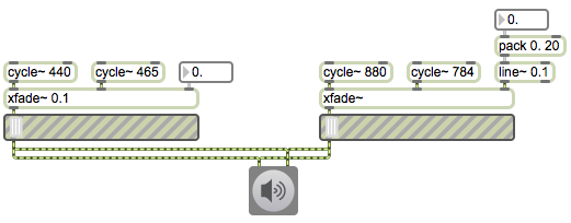
This example demonstrates two ways to establish the initial crossfade value of the xfade~ abstraction. The example on the left uses an initial float argument to establish the initial crossfade value. If you double-click on the xfade~ object on the left, you will see that the two objects that had a #1 argument in the subpatch now have the number 0.1 in those places. This sets up the object so that the cycle~ 440 will have an amplitude of 0.9 in the mix, and the cycle~ 465 object will have an amplitude of 0.1 (about 19 dB lower). The example on the right uses a control signal from the line~ object to provide the crossfade value. So in this case there's no point in typing in an argument in the xfade~ object, because it would not be used by the MSP objects in the subpatch anyway. The argument to the line~ object, however, is important, since it establishes the initial value of that signal. That's where the real initialization takes place for the crossfade value of that xfade~ object.
Notice that the number boxes in these examples show a value of 0 initially, which does not accurately represent the actual initial crossfade value. So if these objects will be presented to the user, and you want them to show the correct value, you would need to initialize them to the value 0.1, too. You could do that with a loadbang object triggering a message of 0.1 or set 0.1.
The gain~ sliders are provided so that you can choose to listen to one or the other of the two halves of this example.
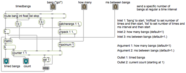
Example 53: Abstraction to trigger a timed series of bangs
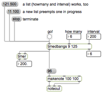
Example 54: Try the timedbangs abstraction
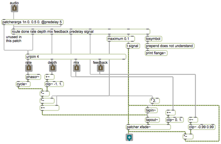
Example 55: Abstraction to flange an audio signal
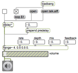
Example 56: Try the flange~ abstraction
Example 57: Introduction to the pattr object
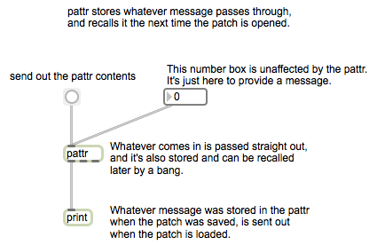
The pattr object and its related objects such as pattrhub, pattrforward, autopattr, and pattrstorage make it possible for you to store data (or any sort of message, really), recall that data when the patch is reopened, store and recall it from other parts of the patch, and make transitions from one set of stored data to another.
The basic unit of storage is the pattr object. It can store any message, its contents will be saved as part of the patch, and it will recall and send out its saved message when the patch is loaded.
Example 58: Binding a pattr object to another object
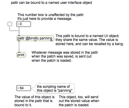
A pattr object can be "bound" to another object, so that the two objects share the same data. By setting the pattr's bindto attribute, you can bind it to any other named pattr object, or a user interface (UI) object that has a scripting name. In this example, we have set the scripting name of the number box at the bottom of the patch to "panning" in the object's Inspector. That allows us to bind it remotely (with no patch cord) to the pattr. (Incidentally, although it's not demonstrated here, you can also bind a pattr to a UI object, even an unnamed one, by connecting the UI object to the pattr's middle outlet.) Once the two objects are bound together, any change to the contents of one of them will be shared by the other, and the contents can be recalled from either of them with a bang. Also, both of them will send out their stored message when the patch is loaded.
Example 59: Binding objects to each other, and to a pattr
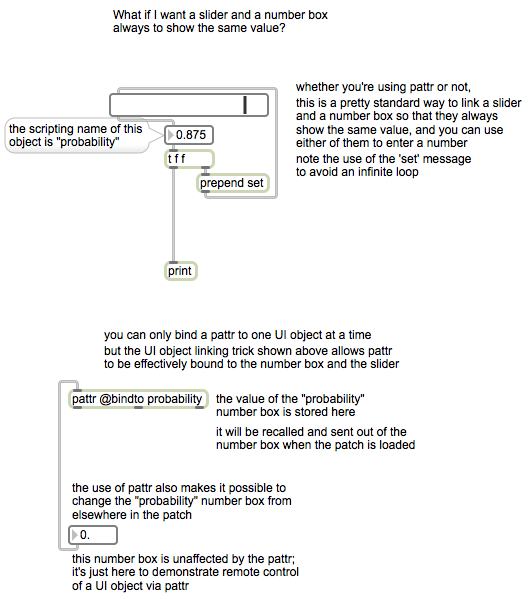
If you want two user interface objects always to display the same information, it might seem sensible to connect the outlet of one to the inlet of the other and vice versa. However, that will lead to an infinite loop unless you do something to stop one of them from always sending out the value. The set message is useful in that regard, because it allows you to set the contents (and the display) of a UI object without causing that object to send out a message of its own. The top part of the patch demonstrates this technique. Whenever the slider is moved by the mouse, it sends its value out to the number box. The number box displays that value and passes it on out its outlet, so both objects end up showing the same (most recent) value. But what if the user changes the number box directly with the mouse? We would want the slider to be updated as well. That's why we use the set message to set the content and appearance of the slider without causing it to send out that value again (which would cause the feared infinite loop). In this way, no matter which object is moved by the mouse, they both correctly show the most recent value.
A pattr can be bound remotely to one of those two UI objects by referencing the object's scripting name (as set in the object's Inspector). Since the two UI objects are bound to each other using the set technique described in the previous paragraph, the effect is as if the pattr were bound to both of those UI objects.
Example 60: Binding pattr objects between a subpatch and its parent patch
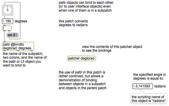
A pattr object can be remotely bound to another pattr or to a UI object, using the bindto attribute, even if one of them resides in a subpatch. To indicate an object in a subpatch, the syntax for pattr's bindto attribute is to use the subpatch name, followed by two colons -- :: -- followed by the name of the object to which you want to bind. Use of that syntax is shown in the pattr in the main patch. Notice that to do this with a patcher object, the patcher needs to have a name typed in as an argument. And of course the object to which you intend to bind needs to have a name, too. If you look inside the patcher degtorad subpatch, you'll see a pattr object with a typed-in name degrees. The pattr in the main patch can bind to it by using the patcher object's name and the name of the pattr object inside the subpatch.
To communicate in the opposite direction, from a pattr in a subpatch to some object in the main patch, you just refer to the patch one level above using the name "parent". In our subpatch, we have a pattr that is bound to the number box named "radians" in the parent patch. (Although it's not demonstrated here, you could even bind objects through multiple levels of subpatches, using multiple :: symbols, as in @bindto parent::parent::radians.)
You may wonder, "Why couldn't we just put an inlet and an outlet in the patcher subpatch, and communicate with it via patch cords?" And you'd be quite right. In this simple example, that would be easier. (But it wouldn't have given us the pretext to discuss the :: syntax.) In more complex situations, you'll see how the ability to bind a pattr to objects on other hierarchical levels can be useful.
Notice how, in this example, the pattr objects in the subpatch have typed-in names, but the one in the main patch does not. We didn't bother to give that pattr a name because no other object needs to bind to it. (It takes care of binding to the degtorad::degrees object all by itself.) As far as Max is concerned, though, all pattr objects have a name. If you don't type one in, Max internally assigns it a quasi-random name.
Example 61: Communicate with many pattr objects from a central hub
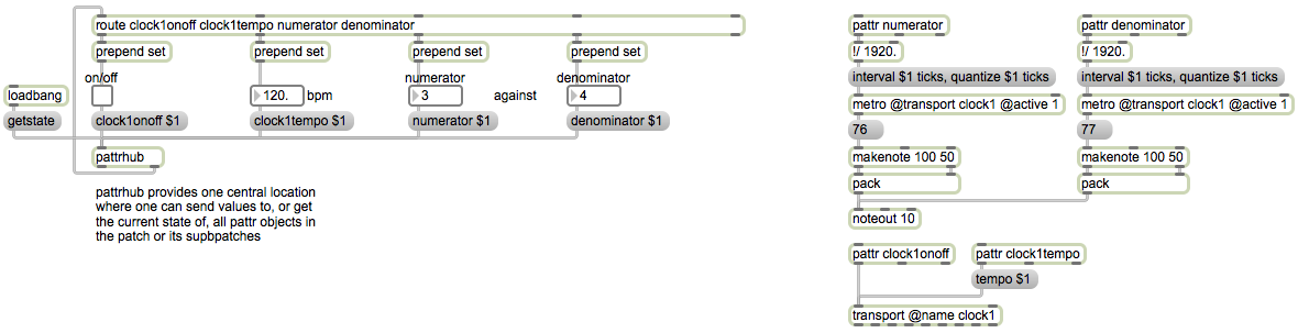
In large and complex patches that have many pattr objects, it might be useful to be able to communicate with all of them at one central location. That is the purpose of the pattrhub object. With pattrhub you can alter the contents of any pattr just by using the name of the pattr followed by the data you want to put in it. You can also query the current contents of any pattr by preceding its name with the word "get" (as in gettempo if there is a pattr tempo object somewhere in the patch). You can query the contents of all the pattr objects in the patch with the message getstate. Whenever you query the values of pattr objects, the information comes out the right outlet of pattrhub, preceded by the name of the pattr(s) in question. Thus, you can use a route object to look for and parse the values of the various pattrs coming out of pattrhub.
In this example, we have made a program that performs simple rational polyrhythms. We specify a numerator and denominator for the ratio of one rhythm to another, and we divide those values into 1920 (the number of ticks in a whole note) to determine the correct number of ticks to use as the time intervals for the two metros. We're using a named transport object, with the name "clock1", to keep it distinct from the global transport. The numerator, denominator, and beat tempo are all stored in pattrs so that we can set them in one part of the patch and use them in another part.
Whatever the values of the pattrs are when the patch is saved, those values will be saved with the patch and will be sent out when the patch is loaded. Using the getstate message to pattrhub, we can query the saved contents of each pattr, and can use that information to set the initial values of the UI objects. Notice that in this case, the pattrs are not explicitly bound to any UI objects, and the UI objects don't have any scripting names. We're just using the getting and setting capabilities of pattrhub to make the communication between the UI objects and the pattrs.
Example 62: Storing and recalling multiple pattr values
[In order for this example to work properly, you should first download the file called twocloudspresets.json and save it with that name somewhere in the Max file search path.]
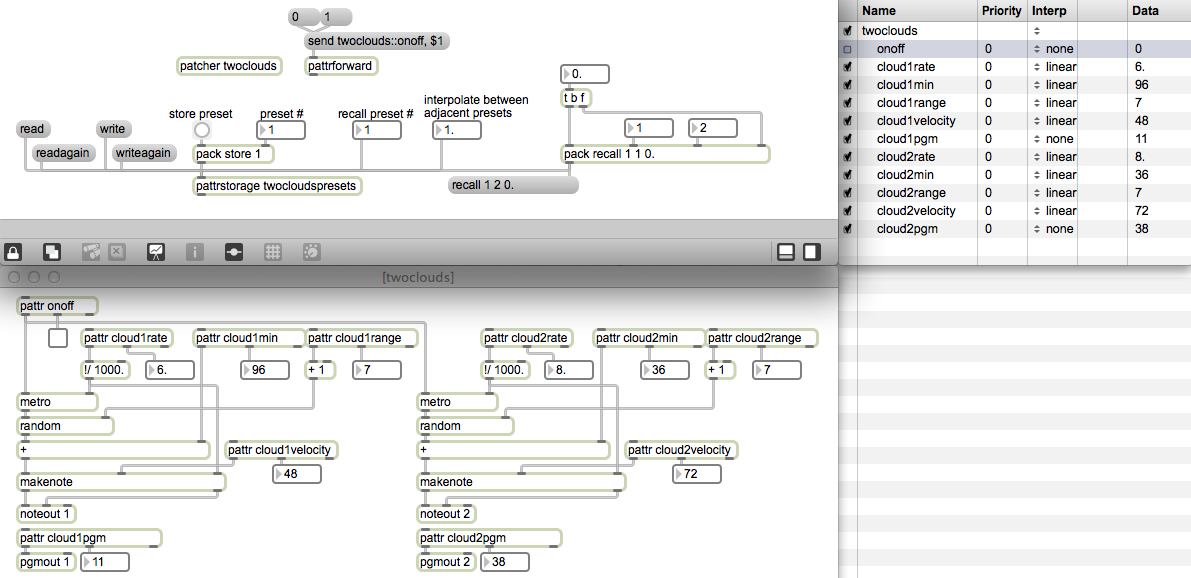
The pattrstorage object allows you to store and recall the states of any and all pattr objects in the patch or its subpatches. Each set of states is stored in a numbered "preset", and pattrstorage can store as many presets as you'd like. The presets can then all be saved in a separate file, in JSON format, and can be loaded in when the patch is loaded. Thus, we can recall any of a number of states for the entire patch at any time. An additional, and very powerful, feature of pattrstorage is that it can interpolate between two different states.
For this demonstration, I made a subpatch called "twoclouds" that generates two streams of MIDI notes. (They're really just two motorhythmic melodies of randomly-chosen pitches. I call them "clouds" because when the melodies are very fast the random behavior is reminiscent of the random movement of particles in a compressed gas.) The parameters that can be controlled are the rate of the notes (notes per second), the loudness (MIDI velocity), the timbre (MIDI program number), and pitch register, which is specified by height (the lowest pitch that can be chosen) and range (how far above the minimum the pitch might be). There is also a pattr bound to the on/off toggle switch, so that the process can be turned on and off remotely. Note that the UI objects attached to the pattrs do not have scripting names, but they are bound to the pattr by the patch cord coming from the pattr's middle inlet. This allows you to see the value of each pattr, and also to modify the contents of each pattr by changing the UI object.
We can store the current state of all the patch's pattr objects in pattrstorage by sending pattrstorage a store message specifying the preset number where we want it to keep the data. In the main patch, we use a pack object to construct the store message. This allows you to choose a preset number, and then click on a button to trigger the store message. (The fact that you have to explicitly click on the button after having specified the preset number in order for anything to be stored helps prevent accidentally overwriting previously-stored presets. If you were simply to use a number box attached to a message box saying store $1, every single number from the number box would cause a preset to be stored.) To recall a preset, all you have to do is provide pattrstorage the number (int or float) of the preset you want to recall.
The preset file "twocloudspresets.json" contains five presets. Use the number box labeled "recall preset #" to choose a preset from 1 to 5. You should see the UI objects in the subpatch change accordingly, showing the values that have been recalled for each pattr. If you don't see that, perhaps the preset file was not loaded properly into the pattrstorage. (When the patch is first loaded, pattrstorage uses its own name to look for a .json file of the same name, but if it can't find such a file, it will contain no presets.) You can read in a preset file by sending pattrstorage a read message. You can also create new presets, if you'd like, by using the UI objects in the subpatch to change the pattr values the way you want them, then storing that data in a pattrstorage preset (presumably in presets 6 and higher). You can then write the presets to a new file with the write message, or directly to the same file with a writeagain message.
One of the most interesting aspects of pattrstorage is its ability to calculate pattr data that is somewhere in between two presets, using a process of interpolation between the values in two presets. You can specify an interpolation between two adjacent preset numbers just by using a float value with a fractional part. For example, to get data that is right between the values of presets 1 and 2, you could send pattrstorage the number 1.5. Try using the float number box labeled "interpolate between adjacent presets" to try this out.
If you want to interpolate between non-adjacently numbered presets, the syntax is a bit more complicated. The message should start with the word recall followed by one preset number (let's think of it as preset A) and then another preset number (we'll think of that as preset B) and then a value from 0. to 1. specifying the location between preset A and preset B. A value of 0 is preset A, 1 is preset B, and intermediate values are some degree of the way from A to B. In this patch, you can specify the two presets between which you want to interpolate, and you can then drag on the number box labeled "interpolation between preset A and preset B", from 0. to 1., to trigger well-formed recall messages to pattrstorage.
You can see the current value of each pattr by double-clicking on the pattrstorage object, which opens a "Client Objects" window. Try that. If you want to, you can even double-click on the data values in the client window to type in new values. You can see that you also have a choice of what type of interpolation you want between presets for each pattr. (See the reference page for a description of the different types of interpolation.) Since interpolating between different MIDI program numbers would mean hearing the timbre of every intermediate program number, interpolation doesn't make much sense for those pattrs, so we have set the interpolation for those items to "none". In the leftmost column of the client window, you can also enable and disable the effect of the pattrstorage object on each pattr. Notice that we have disabled pattrstorage's control of the pattr onoff object in the "twoclouds" subpatch, because we don't want that to be affected by preset changes. We'll control that separately by another means.
In the main patch, you see yet another useful object, pattrforward. By sending pattrforward the word send followed by the name of a pattr, you can set the destination for that pattrforward object. Then any subsequent messages to pattrforward will be forwarded to the named destination. So in our case, each time we click on the message boxes saying 0 or 1, the message will be forwarded to the pattr onoff object in the "twoclouds" subpatch. This shows yet another way to communicate remotely between main patch and subpatch.
Try out a few of the presets, try interpolating between presets, and if you'd like, try creating, storing, and recalling new presets of your own making.
Example 63: Using the preset capabilities of pattrstorage
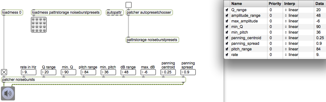
[In order for this example to work properly, you should first download the file called noiseburstpresets.json and save it with that name somewhere in the Max file search path.]
This patch shows some features of pattrstorage, and demonstrates how it might be used to structure a series of different settings to shape the formal structure of a longer period of time.
The first thing to notice is that there is not a single pattr object anywhere in this patch. However, each of the nine labeled number boxes that provides parameter data to the patcher noisebursts subpatch has been given a scripting name in its object Inspector. The autopattr object, as soon as it is created, finds not only all the pattr objects anywhere in the patch but also all the UI objects that have scripting names, and it makes available all of those names -- pattr object names and UI scripting names -- to any pattrhub, pattrforward, and pattrstorage objects in the patch. So, without needing any pattr objects or explicit bindings, all we need to do is include an autopattr at the top level of our patch, and automatically all the UI objects that have scripting names will be storable and recallable by pattrstorage.
The sonic/musical function of this patch is to generate different randomized patterns of short bursts of filtered noise. The patterns are generated inside the patcher noisebursts subpatch -- and all the MSP objects that create the actual bursts of filtered noise are isolated in another subpatch within that so that they can be easily enabled and disabled to turn the sound on and off -- but the UI objects that provide the parameters that shape the noiseburst patterns are all in the main patch. Those UI objects all have scripting names, so they can be controlled by the pattrstorage object, and the pattrstorage can in turn be controlled by the preset object.
Before the whole system of pattr-related objects existed, a standard way to store the settings of all UI objects was with a preset object. (You can see the standard usage of the preset object in action in an example from one of the original Max tutorials, and another good example can be found in the tutorial patch for MSP Tutorial Chapter 7.) The preset object was notoriously a bit buggy and problematic, so the pattrstorage system is ultimately superior. Nevertheless, the straightforward graphic interface of the preset object is very effective, so a feature was added to it that would allow it to be used with pattrstorage. All you need to do is create a preset object, then send it a pattrstorage message indicating the name of the pattrstorage object you'd like it to control. From then on, you can use that preset object to store and recall presets in the named pattrstorage.
When the patch is loaded, the pattrstorage object tries to load in the JSON preset file of the same name, called "noiseburstpresets.json". If you have saved that file correctly in a location that's findable by Max (i.e., within the Max file search path), that should happen automatically. Because the preset object is bound to the pattrstorage object, You should be able to choose different settings for the parameter UI objects just by clicking on different buttons of the preset. Note that the preset is not controlling those objects directly, as it would in a traditional usage of the preset object; it is controlling the pattrstorage object, which is actually in charge of controlling all the UI objects that have scripting names. You can double-click on the pattrstorage object to see its "Client Objects" window. Note that the on/off toggle does not have a scripting name, so it's invisible to the pattrstorage; that's intentional, so that we can turn the sound on and off independently of any preset changes we might make.
Click on the ezdac~ to turn MSP on, use the toggle to turn the noisebursts on, then try choosing one of the 16 saved presets to change the sound.
There is also a subpatch called patcher autopresetchooser that's intended to demonstrate one possible approach to automating preset changes and preset interpolations. Double-click on it to see its contents. The subpatch is designed to choose a new preset number every 15 seconds, form a recall message that will enable interpolation from the previous preset to the newly chosen present, and then trigger a 5-second interpolation from the old preset to the new preset. The resulting messages will thus say recall <previouspreset> <nextpreset> <interpolationvalue>, with each message having a different interpolation value progressing from 0 to 1 over five seconds. Try turning on the "autopresetchooser" subpatch to cycle randomly through all the different presets. This demonstrates how one might automate changes over a long period of time to create a certain formal structure, one that is either determinate or, as in this case, indeterminate because of randomized decisions.
The composition of known states of a patch, governing its behavior, can be composed in non-real time and stored in a whole collection of presets within pattrstorage, and those presets can then be recalled interactively or automatically in a performance to recreate known behaviors at the desired time.
This page was last modified June 2, 2013.
Christopher Dobrian, dobrian@uci.edu