Computer Music Composition and Production

Programming Examples

Programming examples for the class
Music 215A: Computer Music Composition and Production - Winter 2018
University of California, Irvine

This page contains examples and explanations of techniques of computer music programming using Max.

The examples were written for use by students in the Computer Music Composition and Production course at UCI, and are made available on the WWW for all interested Max/MSP/Jitter users and instructors. If you use the text or examples provided here, please give due credit to the author, Christopher Dobrian.

While not specifically intended to teach Max programming, each chapter of Christopher Dobrian's algorithmic composition blog contains a Max program demonstrating the chapter's topic, many of which address fundamental concepts in programming algorithmic music and media composition.

Please note that all the examples from the years prior to 2009 are designed for versions of Max prior to Max 5. Therefore, when opened in Max 5 or 6 they may not appear quite as they were originally designed (and as they are depicted), and they may employ some techniques that seem antiquated or obsolete due to new features introduced in Max 5 or Max 6. However, they should all still work correctly.

[Each image below is linked to a file of JSON code containing the actual Max patch.
Right-click on an image to download the .maxpat file directly to disk, which you can then open in Max.]

Max Examples

Examples will be added after each class session.

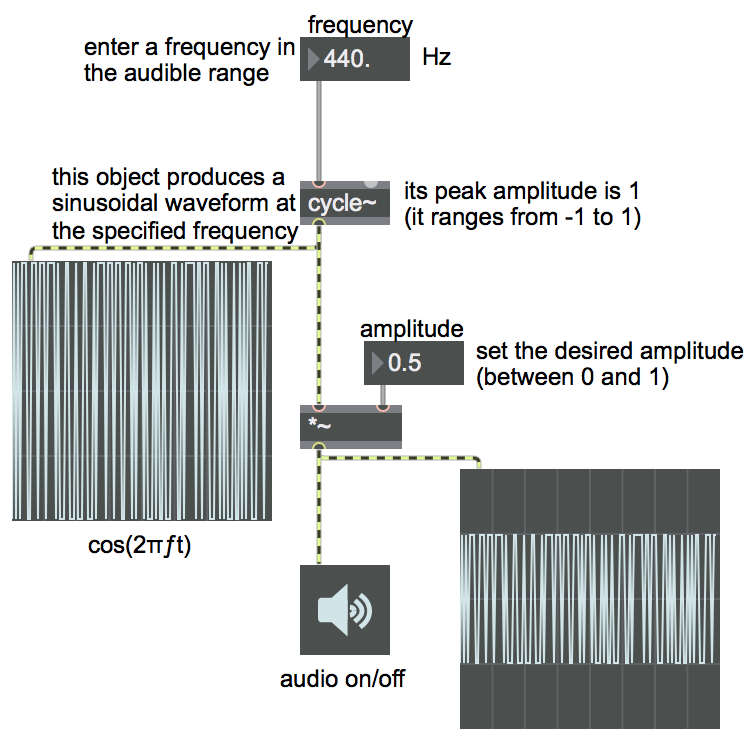
Example 1: Play a sinusoidal tone

This simple program allows you to listen to a sinusoidal tone with any desired frequency and amplitude. Initially both frequency and amplitude are set to 0, so you'll need to set the frequency to some number in the audible range, and you'll need to increase the amplitude to some value greater than 0 but not greater than 1. The speaker icon (ezdac~ object) is an on/off button for audio, and sends the output signal to the DAC.

[If you're totally new to Max, you might benefit from the professor's 15-minute video walkthrough of this example.]

Example 2: Addition of sinusoidal tones

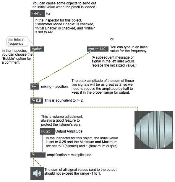
To play two tones, you need two oscillators: two cycle~ objects). To mix them together, simply add the two signals with a +~ object. (For digital signals, addition is mixing.) To control the amplitude, multiply it by some factor, using a *~ object. (Multiplication is amplification.)

Note the psychoacoustic effect of mixing sine tones with two different frequencies. When two tones have nearly the same frequency, we tend to hear only one pitch, but the waves interfere in a way that causes puslation ("beating") at a rhythmic rate up to about 12 times per second. Once the tones are sufficiently far apart in frequency, we can begin to distinguish two pitches and the beating becomes a sort of "roughness", too fast for us to hear as a rhythm. The roughness persists up to about an interval of a minor third, at which point the interval is heard as less rough, more "consonant".

The comments in this patch explain the use of a typed-in "argument" in an object box to set an initial internal value for that object (such as the initial frequency value 440 typed into one of the cycle~ objects), and also describe the use of certain settings in a flonum~ (floating point numberB> box) object's Inspector to cause it to display and send out a specific numerical value when the patch is opened.

Example 3: Multiplication of sinusoidal tones

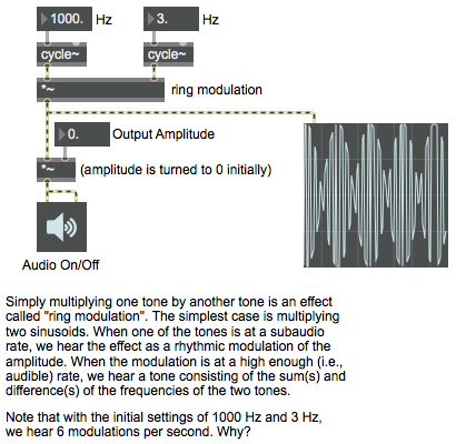
Multiplying one tone by another, in effect, imposes the contour of one waveform on that of the other waveform. For example, mutiplying a 1000 Hz sinusoidal tone by a 3 Hz sinusoidal tone yields something very much like a 1000 Hz sine tone, but with its amplitude continually shaped by the low-frequency oscillator (LFO). Because the LFO goes from 0 to 1 to 0 to -1 to 0 each cycle, the amplitude of the 1000 Hz tone goes from 0 up to 1 and back down to 0, then to -1 and back to 0 for each cycle of the LFO. We don't distinguish auditorily between negative and positive amplitudes, so to us it sounds like the sound is pulsating twice per cycle of the LFO, which, with a 3 Hz LFO, is 6 times per second.

An important fact about multiplication (ring modulation) of two sinuosoids is that the result is mathematically equivalent to adding two half-amplitude sinusoids at the sum and difference frequencies of the two tones. That is, if you multiply a 1000 Hz sinuosoid and a 3 Hz sinusoid, the result is a 1003 Hz sinusoid (the sum of the two frequencies) and a 997 Hz sinusoid (the difference of the two frequencies). The difference between those two tones is, of course, 6 Hz, which is another way of understanding the 6 Hz beating effect.

Ring modulation is a particularly useful effect when one of the two tones is a complex tone containing many frequencies; the modulation creates a sum and difference frequency for each of the component frequencies, radically changing the harmonic content of the tone.

Example 4: Amplitude modulation of sinusoidal tones

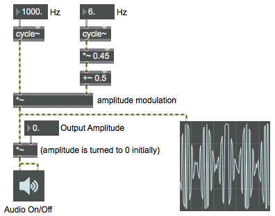
Amplitude modulation is the use of one oscillator—usually but not obligatorily at a sub-audio frequency—to modify the amplitude of a sound. (Ring modulation, shown in example 3, is one particular example of amplitude modulation.) The modulating oscillator is added to a main amplitude value to create an amplitude that fluctuates up and down from the central value. The result, at low modulation frequencies, is called "tremolo".

In this example, the modulating oscillator on the right (with a frequency of 6 Hz, initially) has an amplitude of 0.45, and that output is added to a constant value of 0.5. The result is a value that fluctuates sinusoidally between 0.05 and 0.95 six times per second, without ever going to 0, which is used to control the amplitude of the audible oscillator.

Example 5: Frequency modulation of sinusoidal tones

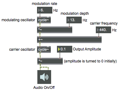
Frequency modulation is the use of one oscillator—usually but not obligatorily at a sub-audio frequency—to modify the frequency of a sound. The modulating oscillator is added to a main frequency value to create a frequency that fluctuates up and down from the central value. The result, at low modulation rates, is called "vibrato".

In this example, the upper oscillator, known as the modulator, is multiplied by 13 and offset (by addition) by 440, so that it goes from 427 to 453. That value is used to control the frequency of the other oscillator (known as the carrier) up and down around the central value of 440, creating a 6 Hz frequency vibrato. Even though the frequency of the carrier oscillator is almost never exactly 440 Hz, the fluctuation is both small enough and rapid enough (+ or - about an equal-tempered quarter tone, six times per second) that we hear the central frequency as determining the pitch of the tone.

When the modulation rate is increased into the audio range, the frequency modulation creates sum and difference tones above and below the carrier frequency in multiples of the modulation rate, while also leaving the carrier tone. If you set the modulation rate to 110 Hz, for example, and increase the modulation depth, you'll get not only the carrier frequency of 440 Hz, but also 330 Hz, 550 Hz, 220 Hz, 660 Hz, 110 Hz, 770 Hz, etc., resulting in a rich complex tone with a fundamental frequency of 110 Hz.

Play around with different values for rate and depth of vibrato to get different effects. If you want, you can watch this video, which does that for you and explains how this example works.

Example 6: Phasor as control signal

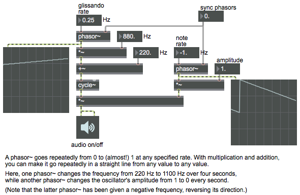
The phasor~ object is an oscillator that makes a "sawtooth" waveform, repeatedly ramping from 0 to 1. (Technically, it goes from 0 to almost 1, because whenever it would arrive at exactly 1, it wraps around and begins again from 0.) You can listen to this sawtooth waveform, but phasor~ is perhaps even more useful as a control signal, to provide a repeated linearly-changing value in your program. You can change its values by multiplying its output (thus scaling it to any desired range) and adding an offset to it to move its range up or down.

In this example, one phasor~ is used to control the frequency of a cycle~ object, and another phasor~ is used to control the amplitude of the cycle~. The first phasor~ is initially given a rate of 0.25 Hz, which means it will complete its ramp every four seconds. The output of that phasor~ is multiplied by 880 and offset by 220, so that it ramps repeatedly from 220 to 1100, and that values is used as the frequency of the cycle~. The other phasor~ has been given a negative frequency, causing it to ramp backward from 1 to 0 once every second. The result is a new amplitude attack every second, while the pitch glides upward over the course of four seconds.

Example 7: Phasor lookup in cosine

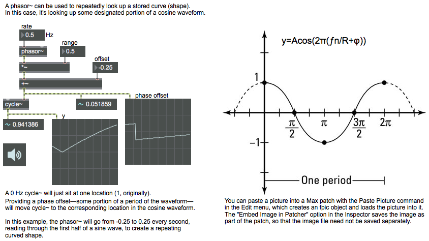
One common usage of the phasor~ object is to readrepeatedly through a stored table of numbers. In that way, instead of just producing a simple linear ramp shape, phasor~ can actually be used to produce any shape. In this example, we're using it to read repeatedly through one half of a sinusoid, so that we repeatedly get just the positive half of a sine wave.

The cycle~ object actually uses a stored wavetable containing one period of a cosine waveform, and reads through that repeatedly at the specified frequency, as if it had its own internal phasor. But instead of using the cycle~ object's internal phasor, you could use a stopped (0 Hz) cycle~ object just for its wavetable, and use the phasor~ to read through a portion of it, via the right (phase offset) inlet.

Example 8: Expanding vibrato on an ascending glissando

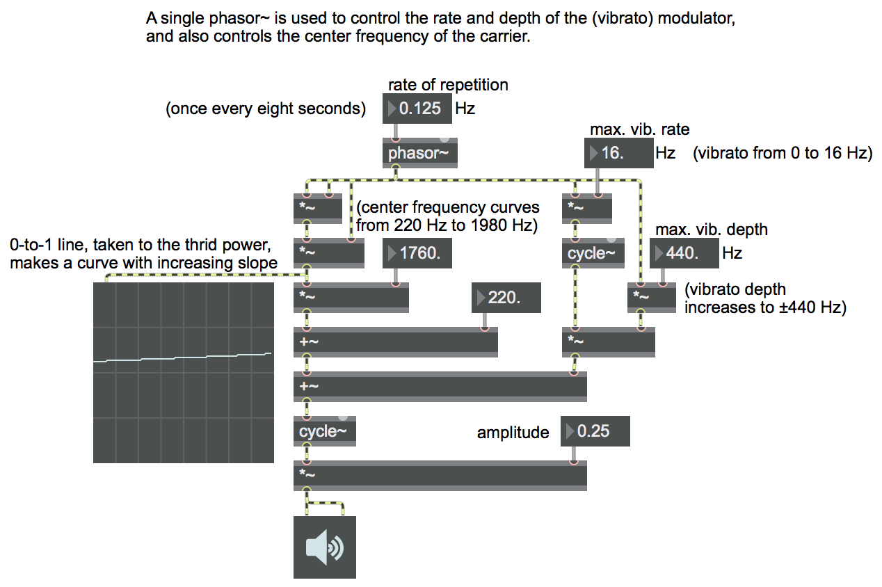
A single phasor~ object can serve to synchronize several different modulations. In this example, the phasor~ is scaled and applied in three different ways. On the left side of the patch, the output of the phasor~ is cubed (multiplied by itself, then multiplied by itself again) so that it's a gentle curve instead of a straight line; that curve is then scaled by a factor of 1760, offset by 220, and used as the central frequency of the cycle~ object. On the right side of the patch, the phasor~ is used to control both vibrato rate and vibrato depth of a modulating cycle~ object; so, in that case, the phasor~ has an indirect effect on the sound, modulating the rate and depth of another modulator. Because all of the modulations are synched to the same phasor~, they all recur with the same periodicity, but the accumulated effect of them makes the sound evolve within each period, creating a tone that rises in frequency while its vibrato increases in rate and depth.

Example 9: Rhythmically out-of-sync phasors

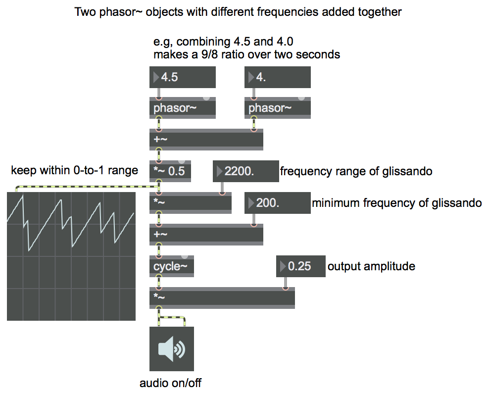
Two low-frequency phasor~ objects with slightly different frequencies can create a rhythmic pattern determined by the ratio of the periodicities of the two LFOs. As an example, this patch uses two phasor~ objects with a frequency ratio of 4.5:4, which, when added together, create a 9:8 rhythmic ratio that repeats every two seconds. That pattern is scaled and offset and used to provide frequency information to a cycle~ object, which is being used as the carrier oscillator. The result is a jagged glissando with a particular pattern and rhythm. If the frequencies of the two phasor~ objects are changed to a different ratio relationship, a different pattern will result.

Example 10: Irrationally out-of-sync phasors

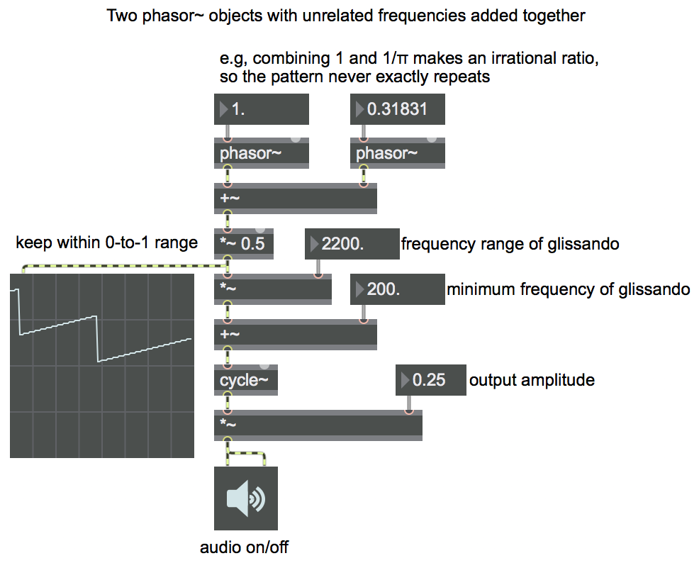
Two oscillators with a ratio of frequencies that's an irrational number will never have exactly the same phase relationship. So, phasor~ objects that have an irrational frequency relationship, when combined, will create a rhythm that never exactly repeats. In this example, you can hear that the sum of the two phasor~ objects with a constantly changing relationship will create a constantly changing rhythm.

Example 11: Hanning function to control parameters of a sound

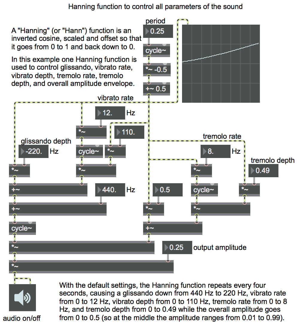
If you scale a one cycle of cosine wave by a factor of -0.5 and offset it by 0.5 you get a "Hanning function", which goes from 0 to 1 and back to 0 as smoothly as possible. That can be used to shape the amplitude of a sound, turning it on and off smoothly, or it can be used to modulate any characteristic of the sound. In this example we use a cycle~ object to generate a Hanning shape that repeats every four seconds (has a repetition rate of 0.25 Hz), and apply that to modulate several characteristics of a sound: center frequency, vibrato rate, vibrato depth, amplitude, tremolo rate, and tremolo depth.

Hanning function

Example 12: Many unrelated LFOs

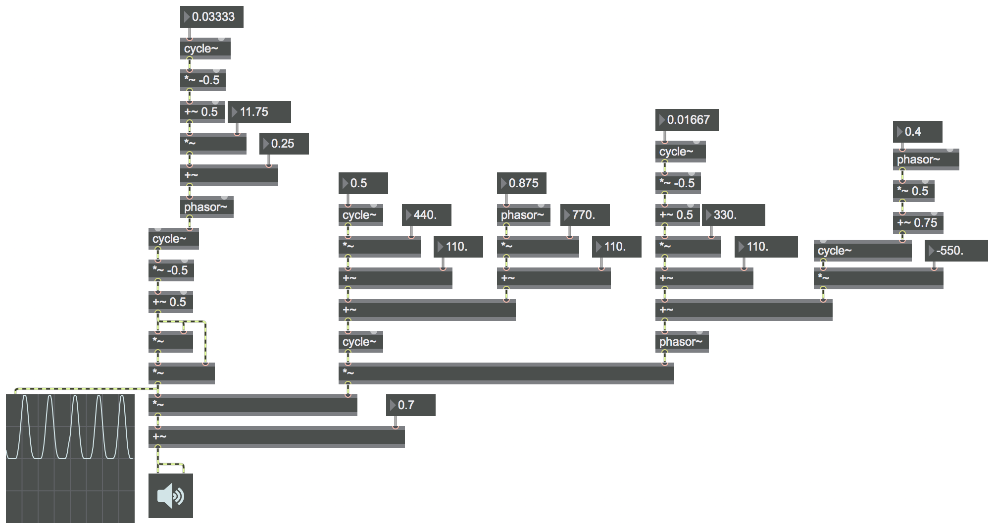
By combining numerous low-frequency oscillators with unrelated repetition rates, you can create irregular shapes of modulation and patterns that never exactly repeat, creating a sound that changes in ways that seem constantly varying in somewhat unpredictable ways. In this example, on the right side of the patch LFOs are combined to create irregular shapes, which control the frequency of a cycle~ object and a phasor~ object, which in turn are multiplied (ring modulation), creating a rich and constantly changing sound; meanwhile, on the left side of the patch an extremely low frequency LFO at a rate of 1/30 Hz (a repetition period of 30 seconds) controls the rate at which a phasor~ object reads through a Hanning function to create note lengths that range from 4 seconds to 1/12 of a second.

Example 13: Open a sound file and play it

See this example from a previous class.

Example 14: Preload and play sound cues

See this example from a previous class.

Example 15: Trigger sound cues from the computer keyboard

See this example from a previous class.

Example 16: Using Presentation Mode

See this example from a previous class.

Example 17: Tremolo by amplitude modulation

See this example from a previous class.

Example 18: Flanging a sound file by modulating the playback rate

See this example from a previous class.

Example 19: Schedule events in the future

In Max, the message bang is used as an all-purpose triggering message, to cause some event to happen. Most Max objects understand the message bang to mean "do whatever you do". In other words, the message bang is used to cause some event (such as playback of a sound file) to occur.

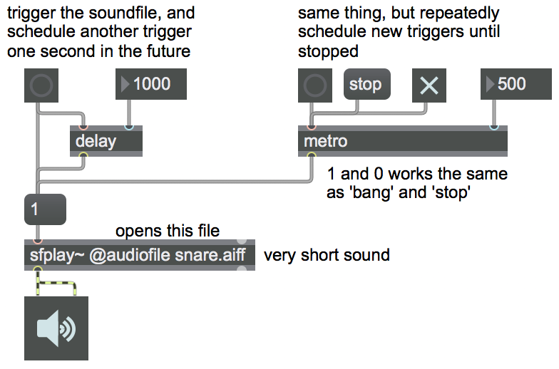
One very important ability for making music, and one of the things that makes Max such a useful program for making music, is the ability to schedule events in the future. "When I do thing A, thing B should happen a specific amount of time later." The Max object that does that is called delay. It receives a bang in its left inlet, and delays that message by the number of milliseconds that has been specified in its right inlet.

Another thing that's important to be able to do in music is cause things to happen at regular time intervals. (In a sense, that's pretty much the same as scheduling something to happen in the future, then at that new time scheduling it to happen again the same amount of time in the future, and so on.) The Max object that does that is called metro, as in metronome. When it gets a bang (or any nonzero integer) in its left inlet, it sends out a bang immediately and also schedules another bang to be sent out some number of milliseconds later, as specified in its right inlet, and does that repeatedly until it receives a stop message (or the number 0) in its left inlet.

This patch shows an example of delay and metro being used to schedule events. The button in the top left of the patch triggers soundfile playback (the message 1), and also tells delay to schedule a bang for one second in the future, which will be used to trigger the same sound event, but it could potentially be used to trigger something else. The button (or the toggle) above the metro object will turn on the metronome, which will send out a bang immediately and will continue to do so every half second until stopped by the stop message or by the toggle.

In these examples, the bang messages are used to trigger a snare drum sound, but you can potentially use a bang to trigger anything, even to turn on a whole other program.

An example from a previous year's class shows the same thing, and also has links to some further readings on the subject.

Example 20: Trigger musical notes with metro

See this example from a previous class.

Example 21: Linear control signal

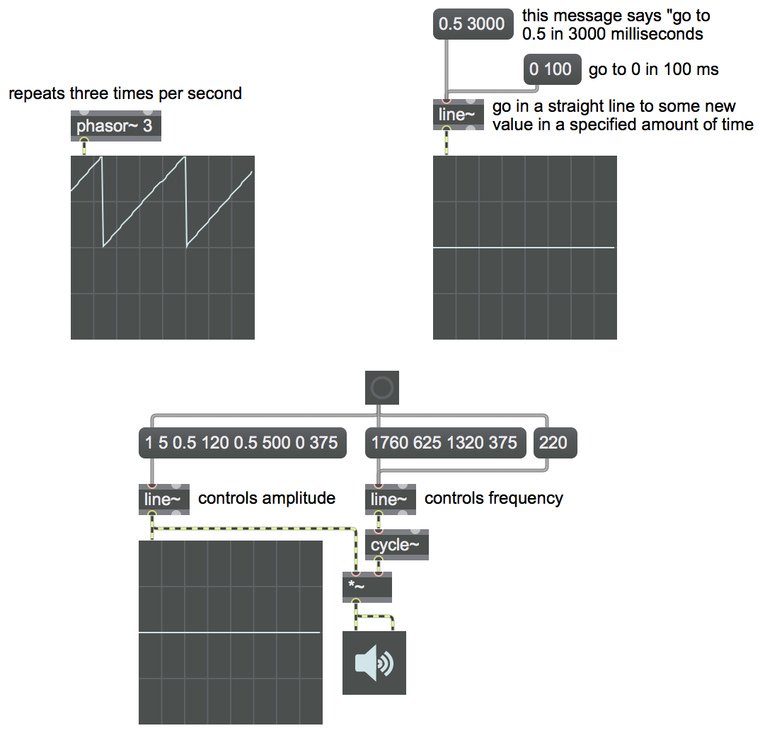
The phasor~ object, introduced in Example 6 above, produces a linear control signal that goes repeatedly from 0 to 1. That's demonstrated in the upper left part of this patch. In general, a control signal that goes gradually in a straight line from one value to another is quite useful, but you don't always want it to repeat over and over the way that phasor~ does.

The line~ object, shown in the upper right part of this patch, produces a control signal that goes from one value to another in a specified amount of time and then stays at that new value until it gets further instructions. The message that it expects to receive is a list of two or more numbers. (A list is a specific message type in Max that starts with a number followed by additional items—usually other numbers—separated by spaces.) The first number in the list specifies a destination signal value, and the second number in the list specifies the amount of time, in milliseconds, that line~ should take to get there.

The lower part of the patch shows the line~ object being used to provide control information for the frequency and amplitude of a tone. Note that line~ can understand a list of more than two numbers; it uses the first two numbers in the list as a destination value and a transition time, and then as soon as it arrives at its destination it uses the next pair of numbers in the list to determine its next destination value and transition time. With longer lists, as shown here, you can define a more complex control shape made up of line segments. If line receives just a single number, it goes to that destination value immediately. (It assumes 0 as its transition time in that case.)

The button triggers three messages. Because of the right-to-left ordering rule of Max messages, the message 220 is triggered first, telling line~ to go immediately to a value of 220. The other two messages then tell one line~ object to play a specific two-segment shape of frequency glissando in a cycle~ object, while another line~ object makes a four-segment shape to control the amplitude of that tone.

You can read a similar explanation of line~ in an example from a previous year's class.

Example 22: Timed counting in Max

See this example from a previous class.

Example 23: Providing MIDI note-off messages

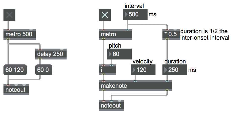
Every MIDI note-on message must be turned off at some time by a subsequent corresponding note-off message for the same pitch (or note-on message with velocity 0). This patch shows two ways to ensure that. One is a very simple way that's illustrative but not ideal; the second way is much more versatile and is the preferred way.

In the left side of the patch, a triggering bang from metro triggers a note-on message on key 60 with velocity 120, and also is delayed for 250 ms before triggering the corresponding note-off to end the note. This is fine, but the delay object can only delay one bang at a time, so it's not useful in more complicated cases, such as in the case of polyphony.

On the right side of the patch you can see a more versatile and more common method, using the makenote object. The purpose of makenote is specifically to provide note-offs to make notes of a specified duration. It can keep track of any number of note-on messages, their pitch and their desired duration, and will provide the corresponding note-off message (actually a note-on message with a velocity of 0) automatically at the correct moment. At each place where there is a number box in this patch, you could be providing changing numbers from some other part of your program, and makenote would keep track of all the appropriate pitches, velocities, and durations and send out the appropriate values to the noteout object to transmit the right MIDI note messages.

Example 24: Playing a pattern

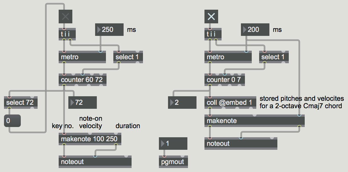
These patches use timed counting—in both cases using a metro object and a counter—to step through a series of MIDI notes.

The example on the left sets the counter to count from 60 to 72, incrementing the count each time a bang is received from the metro. The numbers coming out of the counter are used directly as pitch values, to play a chromatic scale from middle C up to the C an octave above that. A select object is used to detect when the count has arrived at 72, and that triggers a message of 0 to the toggle to turn off the metro.

The example on the right uses the numbers 0 to 7 from a counter to look up pitch and velocity values that are stored in a coll (collection) object. Double-click the coll object to see its contents. Each line of the coll begins with an 'index' number (followed by a comma) that will be used to look up a message, then the message that will be sent out, then a semicolon to end the line. When an index number is received in the inlet of coll, the associated message will be sent out. Because the messages go to a makenote object, the numbers will be interpreted as the pitch and velocity values of a constructed MIDI note-on message. The messages in the coll form a pattern, playing a two-octave arpeggiation of a Cmaj7 chord, with diminishing velocities (i.e. a diminuendo). Because there is no automated stopping condition, the counter will proceed incessantly in a loop from 0 to 7 until the metro is stopped.

Example 25: Program changes for multi-timbral MIDI

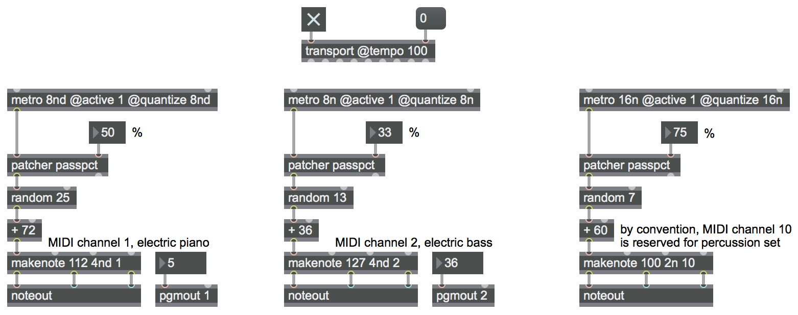
You can use a MIDI "program change" message to tell a synthesizer to change to a different sound. The Max object for that is pgmout.

Note that "program change" is a MIDI channel message, which means that it applies to a particular MIDI channel. Most synthesizers (including the one in your computer's OS) are multi-timbral, meaning that they're capable of playing different timbres on different MIDI channels. So, to get more than one sound at a time, you'll need to send different program change messages on different MIDI channels, and play the notes you want on each channel.

In this example, we've chosen program 5 on MIDI channel 1 (electric piano in General MIDI), program 36 on MIDI channel 2 (fretless electric bass in General MIDI), and some Latin percussion (bongos, congas, and timbales) on channel 10, which by default in General MIDI should be used for key-based percussion set.

Example 26: Beat divisions with the Max transport

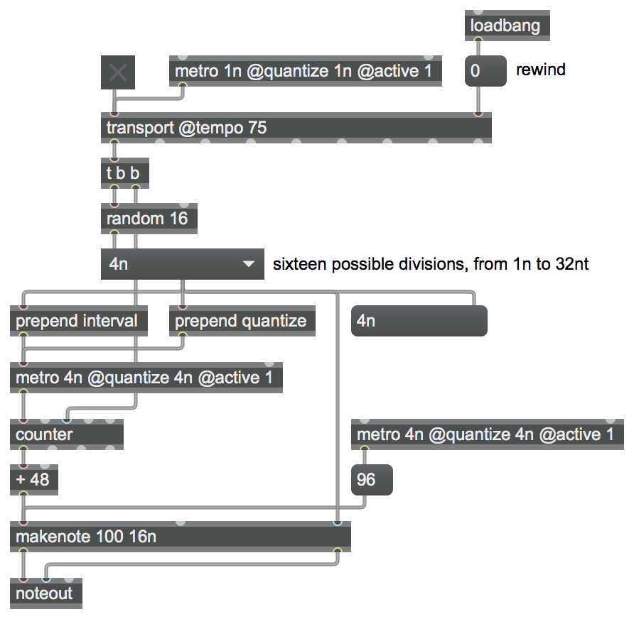
In the MIDI specification, and in most DAW software, and in Max, the smallest unit of metric timing is expressed in "ticks", which is to say, partial units of a beat. Commonly the number of ticks used is 480 or 960 parts per quarter note. That number makes sense because it's divisible by 2, 3, 4, or 5 (and multiples of those).

In Max's tempo-relative timing, there are 480 ticks per quarter note, which means 1,920 ticks per 4/4 measure. There are note value designations for the most common rhythmic values (4n, 8n, 8nt), but not for less-common divisions such as quintuplets and septuplets. For those, you have to use ticks, because there's no note value symbol. For example, quintuplet sixteenth notes (of which there are 20 per measure) take 1,920/20 = 96 ticks each.

Because 7 is mutually prime with 480, there's not an exact number of ticks per septuplet anything. However, internally Max does keep track of ticks as floating-point numbers; you can actually specify fractions of ticks and Max will use the fractional part in its calculations. So, for example, a septuplet quarter note is actually 1920/7=274.285714 ticks. The most precise way to specify ticks for septuplets is to include the decimal part.

In this example patch, a new metrically-related note speed is chosen at random on each downbeat, ranging from whole note (1n) to thirty-second-note triplets (32nt). The divisions, whether expressed as note values or in ticks, are stored in a umenu. One metro triggers a new random choice on each downbeat, and the chosen note value (division of the whole note) is sent to a second metro as its quantized interval, using a counter to play notes of an ascending chromatic scale. A third metro triggers a high note on every beat, to serve as a reference.

Example 27: Trapezoidal control signal

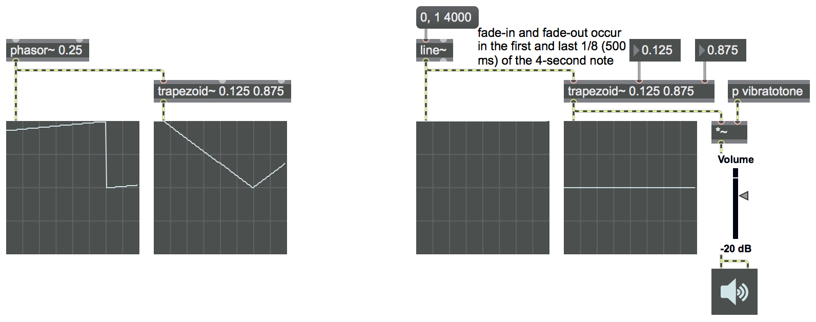
The trapezoid~ object outputs a trapezoidal shape, rising linearly from 0 to 1 in a certain fraction of its time, then staying at 1, then falling linearly back to 0 in a fraction of its time. Its timing is driven by a control signal at its input, one that goes in a straight line from 0 to 1; so a phasor~ or a line~ is the obvious choice for input to trapezoid~. As the input goes from 0 to 1, the output draws the designated trapezoidal shape. (Thus, the ramp times, which are specified as a fraction of the whole period, depend on the timing of the input.)

A trapezoid is often used as an amplitude "window", to create a fade-in at the beginning and a fade-out at the end.

In this example, line~ and trapezoid~ are used to make a 4-second amplitude envelope for a tone. Because the whole envelope is four seconds long, the fade-in and fade-out are each 1/8 of that—500 ms.

Example 28: Simple demonstration of flanging

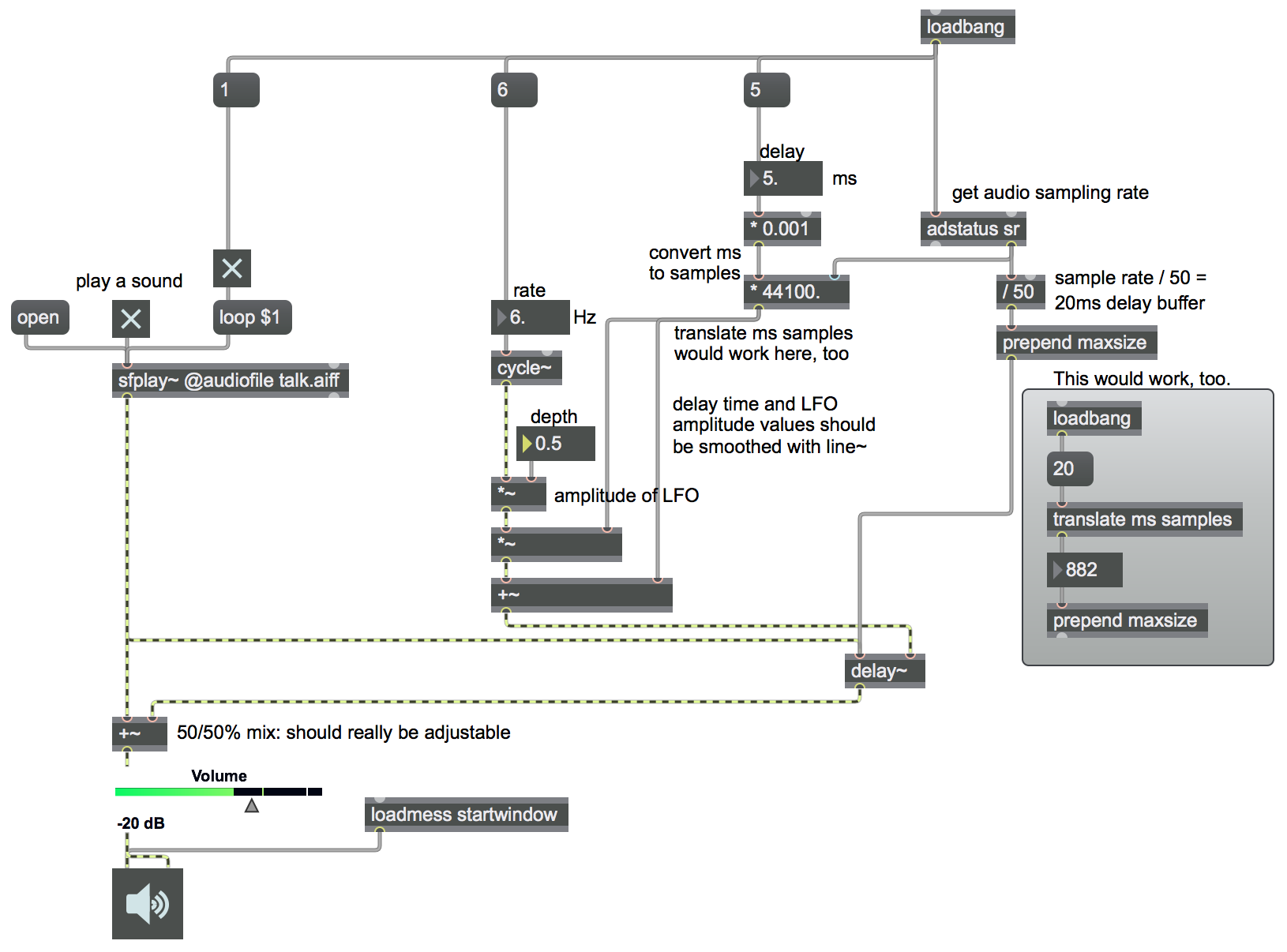
The technique of flanging in computer music refers to a changing delay time applied to a sound, usually by modulating the delay time with a low-frequency oscillator (LFO). The continuously changing delay time causes a subtle—or not-so-subtle—change in the pitch of the sound. When the flanged sound is mixed with the original sound, the two sounds interfere in continuously changing ways, creating a charactistic modulated filtering effect.

This example patch shows how to do that in Max. (A similar take on the same topic can be found in another example of simple flanging.) The idea is to establish a very short delay time (usually not more than 10 ms), and then use an LFO to increase and decrease the delay slightly (again, usually just by a very few milliseconds) at a regular (sub-audio) rate. This creates a pitch vibrato that can range from subtle to extreme.

The sound signal is delayed with the delay~ object, which creates a circular buffer of the most recently received samples of audio, and allows you to specify how much delay should be imposed (provided it's not more than the size of the buffer). The size of the buffer is defined in samples, as is the delay time. The translation between clock time and samples can be done by the translate object, or simply calculated based on the current sampling rate. The rate and depth (frequency and amplitude) of the LFO determine the intensity of the flanging effect.

Some aspects of this patch are oversimplified. For example, changes in delay time and LFO depth should ideally be smoothed (e.g., with a line~ object) to avoid clicks. And the mix between dry sound and flanged sound should ideally be adjustable, rather than fixed in an equal mix as shown here. Improvements to these oversimplifications are demonstrated in the more sophisicated demonstration of flanging.

Example 29: Demonstration of flanging

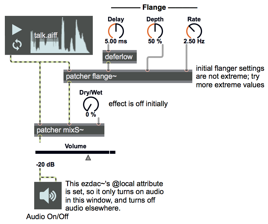
This patch shows an appropriate interface for a flanger, including dials to control delay time, flanging rate, flanging depth, and control over the mix between the dry (unaltered) and wet (altered) signal. Control over the dry/wet mix is a good thing to include in most audio effects.

The live.dial objects give intuitive controls for those important parameters of the effect, and they also limit the range of values that the user can choose from. Note that the left outlet of live.dial sends out the value shown below the dial, while the right outlet sends the dial's position normalized in the range 0 to 1. Both can be useful in certain circumstances, depending on the range of values they need to provide.

You can double-click on the patcher objects to see their contents, and you can drag and drop additional sound files into the playlist~ object if you want to hear the flanging effect applied to other sounds. Try various values for each of the dials, especially extreme values.

This patch has two subpatches encapsulated in patcher objects, which are so generally useful that they could easily be made into abstractions for use in other patches. That's demonstrated in the abstraction for flanging and the abstraction for S-curve mixing.

Example 30: Abstraction for flanging

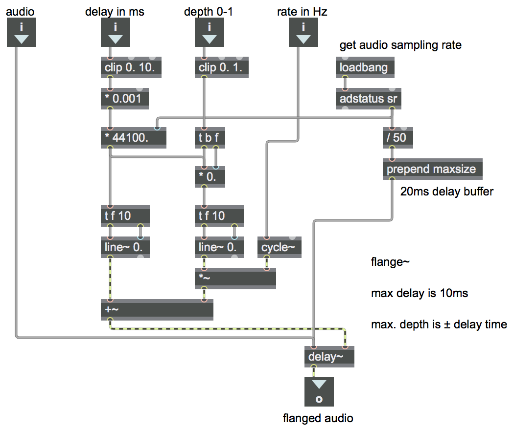
This patch can be used as an abstraction for flanging a sound. It expects to receive values in its inlets to control delay time (limited from 0 to 10 ms), flanging depth (ranging from none at all up to plus-minus the current delay time), and flanging rate in Hertz. It creates a delay buffer of 20 ms in order to accommodate the maximum delay time plus the maximum flanging depth. The delay time at each moment will be a combination of the selected delay and the modulating LFO, translated into samples. You can try out this abstraction in the example that provides a demonstration of flanging.

One feature that's commonly included in flanging algorithms, but that is not implemented in this abstraction, is feedback of the flanged signal back into the input of the delay line. The delay~ object does not allow such feedback. To obtain delay with feedback in Max, one needs to use the objects tapin~ and tapout~ instead of delay~. A similar flanger design, including feedback, with tapin~ and tapout~, is demonstrated in another abstraction to flange an audio signal. Beware, though, because that file and this one are both saved with the name "flange~.maxpat". You should give a different name to one of them (e.g., flangefb~ for the one with feedback) if you want to use both of them.

Example 31: Abstraction for mixing with S-curve law

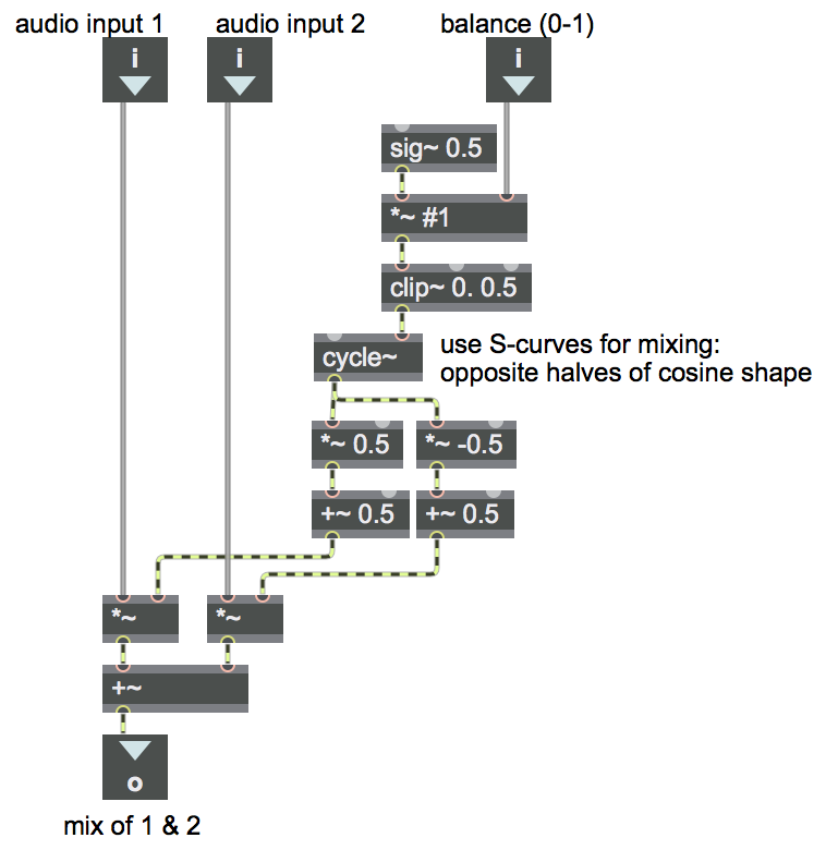
A good way to mix two sounds is to give one sound a gain between 0 and 1 and give the other sound a gain that's equal to 1 minus that amount. Thus, the sum of the two gain factors will always be 1, so the sum of the sounds will not clip. When sound A has a gain of 1, sound B will have a gain of 0, and vice versa. As one gain goes from 0 to 1, the gain of the other sound will go from 1 to 0, so you can use this method to create a smooth crossfade between two sounds. This sort of linear mixing or crossfading is demonstrated in a useful subpatch for mixing and balancing two sounds.

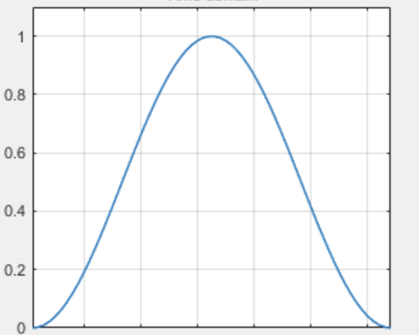
This example does essentially the same thing, except that it uses a non-linear curve for the crossfade. The fade between the two sounds does not go in a straight line from 0 to 1; instead, each sound is faded using half of a cosine waveform. When the two sounds are mixed together, the sum of their gain factors is still 1, which avoids clipping and maintains a constant unity gain, and provides a slightly smoother fade-in and fade-out for each of the two sounds.

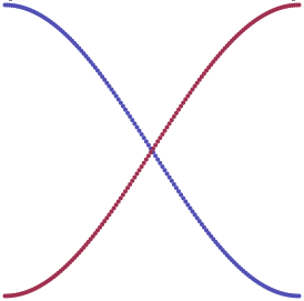
The difference between a straight linear crossfade and this S-curve shaped crossfade (depicted above), is subtle; both are acceptable. The fading curve, calculated by a specific mathematical formula (often referred to as the fade "law"), has a unique effect in terms of the perceived loudness of the sound(s).

Example 32: Mapping MIDI to amplitude

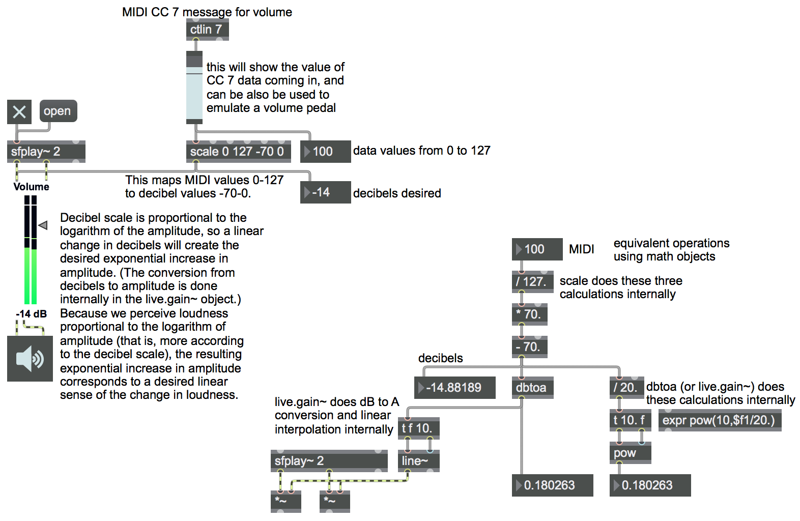
Mapping one range of values to another needed range of values is a crucial technique in computer music. In this example, we want to map MIDI data values that range from 0 to 127 into a useful range for controlling the amplitude—and thus the loudness—of a sound in MSP.

The scale object is the most useful tool for data mapping in Max. The arguments of the scale object are the minimum and maximum input values you expect it to receive, and the corresponding minimum and maximum output values you want it to send out. In this example, in the upper-left portion of the patch, we use as scale object to map input values 0 to 127 (the range of data values from a MIDI continuous control message) into the range -70 to 0 (the default range of decibel values for the live.gain~ object).

If you don't have a MIDI volume controller (a volume pedal or a volume knob or fader on a MIDI device), try dragging up and down on the slider to emulate the effect of a volume pedal. Notice that as the input values go from 0 to 127, the output values go from -70 to 0. In this example the arguments typed into scale are all integers, so the output will be integers. If you want scale to do calculations using decimal numbers (floats), you need to include a decimal point in at least one of the arguments. In this case, we made a quasi-arbitrary decision to use integers, mainly because MIDI data is always integers, and a loudness difference of one decibel is about the smallest change we can perceive anyway, and using integers makes the demonstration simpler.

The live.gain~ object actually does some additional mapping of its own internally. It converts decibels into the amplitude values by which it will scale its audio input. That's exactly the same as the dbtoa or dbtoa~ object would do, combined with a *~ object to scale the amplitude of the sound. Additionally, internally live.gain~ does some rapid smoothing of the amplitude value (linear interpolation from one amplitude to the next) over the course of about 10 ms, to avoid clicks. That's exactly the same as using a line~ object before the inlet of *~.

The lower-right portion of the example patch shows how all of this is working inside the scale and live.gain~ objects, by doing the exact same operations with simple math objects. The incoming MIDI values 0 to 127 are first divided by that full range (127-0=127) to map them into the range from 0. to 1. Then that's multiplied by the desired output range of decibels (70), and then offset by the minimum desired output value (-70) to bring the decibels into the range -70. to 0., as the input data goes from 0 to 127. The dbtoa object shows the conversion from decibels to amplitude. The math objects just to the right of that show what's actually going on inside the dbtoa object. Finally, the line~ object shows the smoothing and multiplication that's going on inside the live.gain~ object after it does the decibel-to-amplitude conversion.

The decibel scale is proportional to the logarithm of the amplitude. That means that a linear change in decibels will create the desired exponential increase in amplitude. Because we perceive loudness proportional to the logarithm of amplitude (that is, we perceive more or less according to the decibel scale), the resulting exponential increase in amplitude corresponds to the desired linear sense of the change in loudness.

Example 33: Constant power panning using table lookup

See this example from a previous class.

Example 34: Abstraction for constant-intensity panning of a monophonic signal to a radial angle between stereo speakers

See this example from a previous class.

Example 35: Abstraction for quadraphonic panning of a monophonic signal, using a left-right value and a front-back value

See this example from a previous class.

Example 36: Abstraction for quadraphonic panning based on radial angle

See this example from a previous class.

Example 37: Abstraction for radial constant-intensity amplitude panning in a hexagonal six-speaker configuration

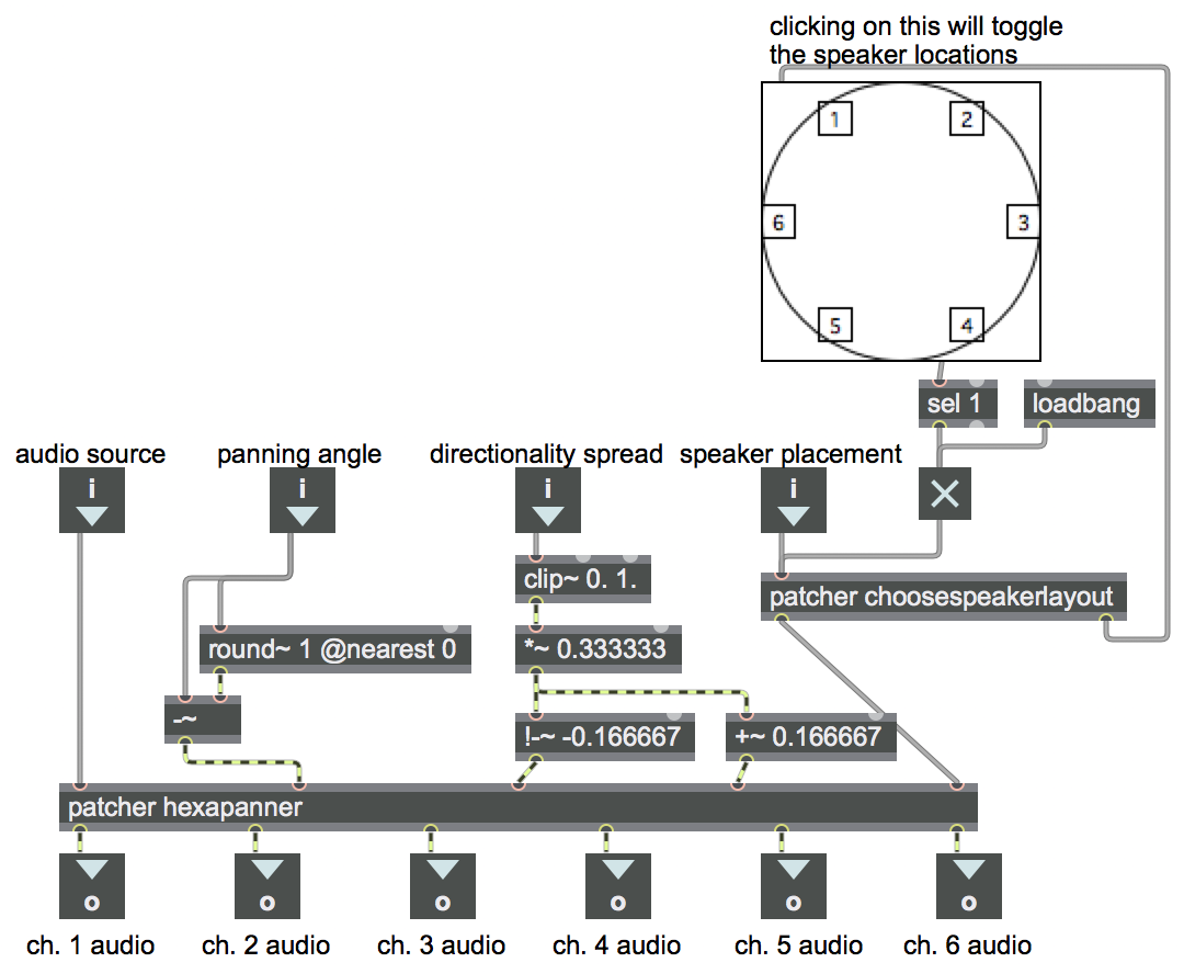
For speakers that are configured in a circle or in the vertices of a regular polygon, you can give a sense of localization of a sound by calculating the radial angle of the sound's desired virtual location relative to the center of the listening space, and then panning the sound between the speakers that are closest to that virtual location. In other words, for any virtual location that you want to imply, you need to calculate which speakers are closest to that location, and then pan the sound between those speakers.

This patch provides a useful abstraction for amplitude panning among a circular (i.e., hexagonal) configuration of six equally-spaced speakers surrounding the listening area. The patch by default assumes that the speakers are equally spaced around the listener at 60° intervals, starting with speaker 1 at -30° to the left off axis from the direction the listener is facing (e.g. in the front-left 11 o'clock position) and with the speaker numbers proceeding in clockwise order from there.

The left inlet receives the sound you want to pan, and the second inlet recieves the azimuth angle to which the sound should be panned, specified as a signal from 0 to 1. (Numbers in the form of Max float messages must be converted to a signal with sig~ or line~ before being sent in the panning inlet.) The use of the range 0 to 1 is agnostic regarding units such as degrees or radians, and makes it easy to pan the sound in a repeating circle using a phasor~ object for the panning angle.

The source sound's panning angle, 0 to 1, is stated as a fraction of a circle, starting from 12 o'clock and increasing in a clockwise direction. As the panning angle enters the range of each speaker (within 60° on either side of the speaker), the amplitude of that speaker increases to 1 using the first 1/4 of the sin function. As the panning angle moves away from that speaker's angle, the amplitude decreases using the first 1/4 of the cos function.

The third inlet receives a signal from 0 to 1 specifying a "spread" beyond the two closest speakers (i.e., beyond the 120° range described in the preceding paragraph). The default spread (spread value of 0) will use just two of the six speakers at any given moment. A spread of 0 to 0.5 will inreasingly use the four nearest speakers, and a spread of 0.5 to 1 will use all six speakers.

The fourth inlet takes an integer 0 or 1 specifying one of two speaker placement options. The default (1) is as described above, with front left and right speakers, left and right side speakers at -90° and 90°, and rear left and right speakers, and with the speakers (output channels) numbered starting with the front left speaker and increasing in the clockwise direction. The other option (0) rotates that configuration by 30 degrees, so that speaker 1 is directly in front of the listener.

With this abstraction, a single signal from 0 to 1 can specify the azimuth angle of the sound. (Any panning signal value outside the range 0 to 1 will be wrapped around to stay within that range.) The virtual distance (D) of the sound from the listener can be modified outside of the abstraction (before panning) simply by scaling the sound's amplitude by a factor of 1/D.

Example 38: Test the hexagonal radial panner

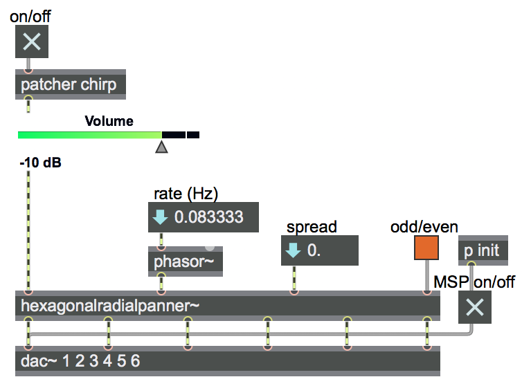
This patch requires the abstraction for hexagonal radial panning to be saved in the Max file search path with the name "hexagonalradialpanner~". It demonstrates the 6-channel panner, and shows how the sound can be moved around the space in a repeating circle by using a phasor~ to supply the panning angle.

An annoying chirping sound, synthesized in the patcher chirp subpatch will be panned clockwise in a circle, at whatever rate is specified by the phasor~ object. (Most likely you'll want the rate to be less than 1 Hz. It should be 1 divided by the number of seconds you want for one revolution around the space. A negative rate will pan the sound in a counter-clockwise circle.)

You can experiment to hear the effect of the "spread" value, from 0 to 1, to diffuse the sound over an increasing spatial range (i.e., give it a less focused directionality). The default spread of 0 will use just two of the six speakers at any given moment. A spread of 0 to 0.5 will inreasingly use the four nearest speakers, and a spread of 0.5 to 1 will use all six speakers.

This page was last modified March 14, 2018.
Christopher Dobrian, dobrian@uci.edu