Example 1: Open a sound file and play it.
This page contains links to explanations and example Max patches that are intended to give instruction on some basic concepts of interactive arts programming using Max.
The examples were written for use by students in the Music Technology course at UCI, and are made available on the WWW for all interested Max/MSP/Jitter users and instructors. If you use the text or examples provided here, please give due credit to the author, Christopher Dobrian.
There are also some examples from the previous years' classes available on the Web: examples from 2010's Interactive Arts Programming class, examples from 2009's class, examples from 2007's class, examples from 2006's class, examples from 2005's class, and MSP examples and Jitter examples from 2004's class.
While not specifically intended to teach Max programming, each chapter of Christopher Dobrian's algorithmic composition blog contains a Max program demonstrating the chapter's topic, many of which address fundamental concepts in programming algorithmic music and media composition.
You can find even more MSP examples on the professor's 2007 web page for Music 147: Computer Audio and Music Programming.
And you can find still more Max/MSP/Jitter examples from the Summer 2005 COSMOS course on "Computer Music and Computer Graphics".
Please note that all the examples from the years prior to 2009 are designed for versions of Max prior to Max 5. Therefore, when opened in Max 5 they may not appear quite as they were originally designed (and as they are depicted), and they may employ some techniques that seem antiquated or obsolete due to new features introduced in Max 5. However, they should all still work correctly.
[Each image below is linked to a file of JSON code containing the actual Max patch.
Right-click on an image to download the .maxpat file directly to disk, which you can then open in Max.]
Examples will be added after each class session.
January 4, 2011
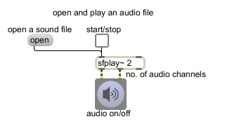
Example 1: Open a sound file and play it.
This shows an extremely bare-bones program for audio file playback.
1. Click on the speaker button (ezdac~ object) to turn audio on.
2. Click on the word "open" (message object) to open a dialog box that allows you to select a sound file. (In the dialog, select a WAVE or AIFF file and click Open.)
3. Click on the toggle object to start and stop playing. (The toggle alternately sends a "1" or "0" to the sfplay~ object, which sfplay~ interprets as "start" and "stop".)
The sfplay~ box is an MSP object. It performs an audio task: it plays sound files from disk and sends the audio signal out its outlets. The number 2 after sfplay~ is an 'argument', giving the object some additional information: that it should play in stereo, and thus should have two audio signal outlets. (The third outlet will send a notifying message when the soundfile is done playing, but this program doesn't use that outlet.) The speaker button (a.k.a. the ezdac~ object) is a 'user interface object'. It allows the user to interact with the program (in this case, by clicking on it with a mouse) and it performs a task (to turn audio on and off, and to play whatever audio signals it receives in its inlets as long as audio is turned on). Notice that the patch cords between the outlets of sfplay~ and ezdac~ are yellow and striped; that indicates that what is being passed between those objects is audio signal. The open object is a 'message box'. It's a user interface object, too. When clicked upon, it sends the message it contains (in this case, the word 'open') out the outlet to some other object. This is a message that sfplay~ understands. (If it were not, sfplay~ would print an error message in the Max window when it received an unfamiliar message.) The plain black patch cord indicates that what is passed between these objects is a single message that happens at a specific instant in time rather than an ongoing stream of audio data. The words 'start/stop' and 'audio on/off' are called comments. They don't do anything. They're just labels to give some information.
Here are a few thoughts for you to investigate on your own.
If you wanted audio to be turned on automatically when the patch is opened, and/or the 'Open File' dialog box to be opened automatically, how would you make that happen? (Hint: See loadbang.)
If you want to cause something to happen when the file is done playing, how would you do that? (Hint: Read about the right outlet of sfplay~.)
If you wanted to play the file at a different speed than the original, how would you do that? (Hint: Read about the right inlet of sfplay~.)
A single sfplay~ object can only play one sound file at a time, but it can actually access a choice of several preloaded sound files. How can you make it do that? (Hint: Read about the preload message to sfplay~.)
Suppose you'd like to be able just to pause sfplay~ and then have it resume playing from the spot where it left off rather than start from the beginning of the sound file again. Is that possible? (Hint: Read about the pause and resume messages to splay~.)
What if you want to start playback from the computer keyboard instead of with the mouse? (Hint: See key -- and/or keyup -- and select.)
Suppose you want to have control over the loudness of the file playback. What mathematical operation corresponds to amplification (gain control)? (Hint: See *~. See also gain~.)
January 6, 2011
Example 2: Preload and play sound cues.
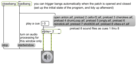
A single sfplay~ object can refer to many different sound files, or even specific portions of sound files, with a unique "cue" number assigned to each sound. Once those sound cues have been preloaded (i.e. taught to the object), you can cause the object to play a cue just by sending the desired cue number in its left inlet.
The open message demonstrated in the previous example can also be used with an argument naming a particular sound file, as in open myfile.aif. This preloads the sound file directly into cue number 1, without using a dialog box to let the user find the file, and subsequently sending the number 1 to sfplay~ will play that file. The message preload followed by a cue number, followed by the name of a file, as in preload 2 my2ndfile.aif, will preload the file and assign it cue number 2, and subsequently sending the number 2 to sfplay~ will play that file.
Note that when you ask Max to find a file for you automatically, Max has to know where to look for that file. How will it know? Read the discussion of Max's file search path in the documentation.
In this example we use the loadbang object to set up some initial conditions in the program. This is an extremely common technique for setting up your program to function correctly and display the correct information when it's first opened. Once the entire program has been loaded into RAM, the loadbang object sends out a bang message, which you can use to trigger the initial conditions and actions that you want. Here we use it to preload all the sound cues we want, and to start up MSP audio processing (i.e., to start generating audio signal) in this program. By so doing, we have taught sfplay~ its 8 sound cues, and we've started sending signal to the computer's sound output. The signal is all 0 until we play a sound cue, but it's on nevertheless, so we're ready to go. Choosing a number other than 0 in the number box will now play the cue.
When the user closes the window, the closebang object will make sure that MSP is turned off with a stop message. This is maybe a good opportunity to discuss the difference between start and startwindow for dac~ and ezdac~. The start message turns on audio processing for the entire Max application, meaning that it's on in all loaded patches. The startwindow message turns on audio processing only for the patch in which the dac~ or ezdac~ object resides, and any subpatches it may contain, but turns audio processing off in all other loaded patches. The stop message turns off all audio processing in all patches. When audio has been turned on in only one window with the startwindow message, audio in all other windows will be turned off, but if you then close the window in which the audio was turned on with startwindow, MSP will be turned back on in the other open windows. So, if you wish to avoid that, and truly have the audio processing be turned off everywhere once that window is closed, a good way to ensure it is to trigger a stop message with closebang, as in this example.
One other tidbit of information relevant to this example is that the comma character in a message box has a special meaning. It serves as a separator of messages. That allows you to include a whole sequence of messages in a single message box. When the message box is triggered (with either a mouse click or an incoming message), the messages are sent out and executed consecutively as fast as possible. So in this example, a single bang actually triggers an open message (to set up cue number 1) and seven preload messages (to set up cues 2 thru 8). If, for some reason, you actually want to send a message that contains a comma, you would have to precede it with a backslash, as in Hey\, how do you like that comma? The backslash is what's called an "escape character" in programming; it's a character that precedes another character to remove that character's specialized meaning and just treat it as a neutral character.
Example 3: Trigger repeated actions metronomically.
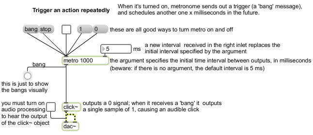
The metro (metronome) object is the most obvious way to trigger repeated events in Max. Repetition is, of course, a key component of most music (and most time-based art in general), and the metro object encapsulates the whole low-level process of a) cause something to happen, b) schedule the same thing to happen at some future time and repeat the process. The only thing it needs to "know" is what time interval to use for its repetitions. You specify that time interval in milliseconds, by an initial argument and/or a number in the right inlet.
For a bit more about timed repetition, you could read my blog article about it.
You many not find milliseconds to be the most musically useful unit with which to think about music, and in fact Max does provide a more music-friendly way to think about time, which you can also read about in a blog article on the subject.
In this example metro doesn't really trigger anything very significant, but you should bear in mind that, since there are many objects that can be triggered by the bang message, a metro could trigger almost anything, including a whole other program.
January 11, 2011
Example 4: Adjusting audio amplitude.
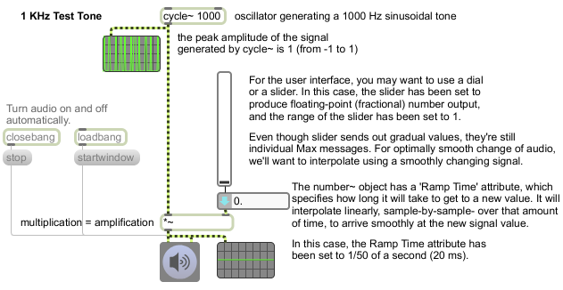
The operation of amplification in audio (turning the volume up or down) corresponds to the mathematical operation of multiplication in your program. If you send a Max message to the *~ object to provide a new multiplier value, the amplitude of the audio signal might change so abruptly as to cause an unwanted click in the sound, as described in MSP Tutorial 2. To avoid such clicks, you need to use a control signal instead, one that interpolates to the new multiplier sample-by-sample over the course of a small amount of time. The number~ object is capable of doing that. It ramps smoothly to a new value over a number of milliseconds that you can specify in the Ramp Time attribute in the object's Inspector. (You can also set the ramp time via the object's right inlet.)
Example 5: Linear fade-in/out of audio.
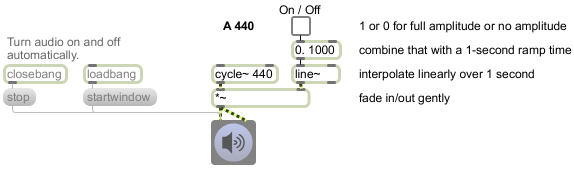
The line~ object is useful for providing a control signal. It interpolates linearly sample-by-sample to a new signal value over a specified period of time, then stays at that new value until it is instructed to change. It expects to receive a transition time in its right inlet (a ramp time), followed by a destination value in its left inlet. Alternatively, you can provide both values as a single two-item list. Its initial default value is 0. In this example, we use line~ to provide a control signal (multiplier) to the *~ object in order to turn the amplitude of a sine wave up and down. When line~ receives the message 1 1000 it progresses to 1 over the course of 1 second, and when it gets the message 0 1000 it ramps back down to 0 in one second.
January 13, 2011
Example 6: Generate MIDI notes.
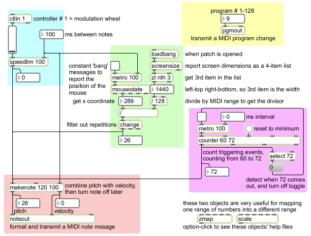
Here are three ways of generating MIDI notes that we discussed in class. Admittedly they don't result in very interesting music, but they show ways how numbers can be converted for usage as pitch information.
At the bottom-left, in the pink portion of the patch, the makenote object receives numbers in its left inlet, considers them to be MIDI pitch numbers, combines them with a velocity value (supplied either as the first argument typed into the object box or as a number received in the middle inlet) and sends them both out. Using the duration value (supplied either as the second argument typed into the object box or as a number received in the right inlet), it schedules a corresponding note-off message to be sent that many milliseconds in the future; at that time it sends out the same pitch with a velocity of 0. The outputs of makenote are designed to go directly to the pitch and velocity inlets of noteout, which formats a MIDI note message and sends the MIDI to an external destination. You can double-click on noteout to choose the destination device. The simplest thing is to send the notes to the built-in DLS synthesizer of your operating system.
At the upper-left, in the blue portion of the patch, the ctlin object looks only for MIDI continuous controller messages with a controller number of 1 coming from an external source. (You can double-click on the object to select the MIDI source.) Controller 1, by convention, designates the modulation wheel of most controllers. The value of each controller 1 message comes out the left outlet of ctlin and is displayed graphically by the slider. You can also generate such values just by dragging on the slider with your mouse. The range of the slider, by default, is 0-127 just like the range of a MIDI controller value. The speed with which those messages come in is determined by the source device. It's often quite fast, say, 50 messages per second. To limit the speed of such a rapid stream of numbers to something more like a human note speed, we use the speedlim object. That object refuses to send out more than one number per time interval (specified by a typed-in argument or a number received in its right inlet). Any numbers that come in faster than that will be suppressed. Drag on the slider to play some notes.
As demonstrated in the upper-right (yellow) portion of the patch, you can change the timbre of the synthesized sound by sending a MIDI program change number via the pgmout object.
In the lower-right (purple) part of the patch, we use a metro to send out repeated triggers at a specified time interval, and we use a counter to count the events as they occur. The exact numbers in the count depend on the specified minimum, maximum, and direction values that have been provided to the counter. (See the counter reference page for details.) In this case, we used typed-in arguments to specify a minimum of 60 and a maximum of 72. We use a select 72 object to detect when the count reaches 72, and when that number is detected we trigger a message of 0 to the toggle to turn it off. The result is a one-octave upward chromatic scale. (Pop quiz: By inserting just one object, can you make it play a whole-tone scale instead?)
The central (green) portion of the patch shows one way you could use the position of the mouse to play notes. The mousestate object reports the location of the mouse (its horizontal and vertical offset, in pixels, from the top-left corner of the screen area) out its second and third outlets every time it receives a bang in its inlet. To keep a constant watch on the mouse position, use a fast-paced metro. Here we use a metro with a time interval of 100 ms so that the maximum note speed will be 10 notes per second. But wait! The horizontal range of pixels on your screen is probably much greater than 0-127. The horizontal dimension of your display is likely 1024 pixels, or 1440, or even greater. So the x coordinates reported by mousestate will likely be in a range such as 0-1439. To solve that problem, we "map" the larger range into a smaller range using arithmetic. The screensize object reports the screen dimensions as a 4-item list noting the left, top, right, and bottom limits of the screen (such as 0 0 1440 900). The zl object is a very useful object for all sorts of operations dealing with lists; here we use it to get the nth number from the list, namely the 3rd number which (assuming that the left boundary is 0) will tell us the screen width. We divide the screen width (the range of possible pixels) by 128 (the range of MIDI note values), and we use that number as the divisor for every mouse x coordinate that we get. (Note that by default the / object will perform integer division and throw away any remainder.) That will reduce the range of numbers we can produce with the mouse to a range from 0 to 127, just as we would like. However, that will likely result in many repetitions because the number of possible mouse locations is much greater than the number of possible notes (and because our metro keeps triggering mousestate even when the mouse is not moving). So, to filter out repetitions, we use the change object, which only lets an incoming number pass through if it's different from the previously received number. Try turning on the mouse-polling metro and playing some notes by moving the mouse on the x axis.
Notice that with the slider (or mod wheel) and the mouse, we're generating numbers that span the full range of all possible notes in MIDI from 0 to 127. That goes from the lowest note C at about 8 Hz (which technically would be a sub-audio fundamental frequency) up to the G a perfect 12th above the top note of the piano (about 12,500 Hz). That's a much larger range than we usually use in most musical situations! A more standard traditional range would be approximately from 36 to 96 (cello low C to flute high C), which is the normal range of a standard 5-octave MIDI keyboard. To perform such a mapping in Max (e.g., mapping the range 0-1439 into the range 36-96), you might want to use the object zmap or scale.
January 18, 2011
Example 7: Delaying MIDI notes.
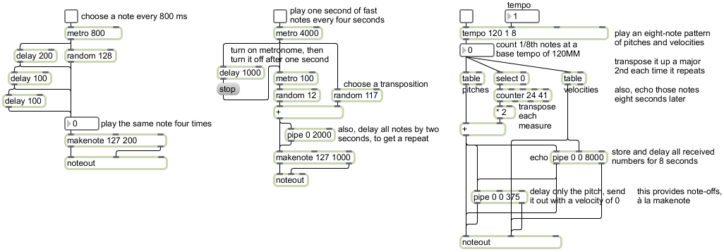
There are many objects available for delaying events (i.e., for scheduling events to happen at a specific future moment). For timing and scheduling events, the most common object is the metro object (send bang periodically at a specified time interval), which can be used to trigger events, start/stop entire processes, or trigger a counter to step through a table or a coll or any sort of sequence of things. To show the user the passage of time, the clocker object is useful (report elapsed time periodically), as are timer (measure the time between two events) and tempo (count rhythmic units according to a metronomic tempo). For delaying a single bang, use delay; for delaying one or more numbers, use pipe; for delaying an audio signal, use delay~ or the variable delay line objects tapin~ and tapout~; for delaying a video, you would generally use jit.matrixset.
This patch contains a couple of simple examples demonstrating the use of delay and pipe (note that one is for bangs and one is for numbers), plus a slightly more complex example using tempo (to look up numbers in a table at a metronomic rate) and pipe (to echo the notes, and also to provide all the note-offs).
The first program, on the left side of the patch, chooses a number at random from 0 to 127 every 800 milliseconds and plays it as the pitch of a MIDI note. Each number gets displayed, and stored temporarily, in the number box. Each bang from metro that triggers a number also gets delayed by three different delay objects, and those delayed bangs trigger the same number in the number box a few tenths of a second later. What results is a 4-note rhythmic pattern for each pitch.
The second program, in the middle of the patch, illustrates a couple of important concepts. The first concept is that timing is an important aspect of a composition at many structural levels: microscopic (the sample level in audio or the frame level in video), small formal level (notes in music or edits in video), middle formal level (such as a phrase in music), or even at the global formal level (entire sections of a composition, scenes, etc.). Thus, a metro object can be used to generate a very fast sequence of bangs to display frames of video or generate a smooth stream of events, and it can be set moderately fast to generate notes, but it can also be set to a much longer time interval to trigger phrases (sequences of notes or events) or to turn on and off entire complex programs. A second concept is that the same bang that triggers the start of a process can also be used to trigger a delay object to turn off the same process at some designated time in the future. Also, perhaps most commonly, delays can be thought of as echos or repetitions, either short-term or long-term, either verbatim or with some sort of variation.
At the top of the program is a slow metro that sends a bang every four seconds. The first thing it does is trigger a random number from 0 to 116, a "transposition" value to be stored as the right operand of the + object. Immediately after that, it turns on a faster metro, and it also triggers a delay object. The faster metro chooses random numbers from 0 to 11 at a rate of ten times per second. Those numbers get added to the randomly-chosen transposition value in the + object and used as MIDI pitch values by makenote. After one second of that, the delay object stops the fast metro, thus ending the "phrase" of fast notes. However, the fast pitch values are also all delayed by a pipe object that passes them on two seconds after they were generated, thus performing an echo of every randomly-generated phrase two seconds later.
The third program demonstrates the use of the tempo object, demonstrates the use of the table object, and also shows two uses of the pipe object.
The tempo object is like a combination of metro and counter, but it allows you to specify its rate in particular music-related terms. The first argument of tempo (or a number in its second inlet) specifies its tempo, in quarter notes per minute. The help file and manual page say that the tempo refers to "beats per minute", but it's really much more correct to say that it refers to quarter notes per minute. That's because tempo is biased toward 4/4 meter. It thinks of a measure always as being a whole note, and its tempo refers to the rate of a quarter note. The next two arguments (inlets) are for specifying a "multiplier" and "division", which are probably best thought of as the numerator and denominator of the fraction of a whole note that you want tempo to use as its actual rate of output. For example, in this program, we have specified a tempo (a quarter note rate) of 120 bpm, and we've asked tempo to report 1/8 notes. At a quarter note rate of 120, we would expect eighth notes to occur at a rate of 240; that is, if quarter notes occur every 500 ms, eighth notes occur every 250 ms. This tempo object thus outputs at a time interval of 250 ms, and counts the eighth notes in the 4/4 measure, starting at 0 (as computers often do) and counting up to 7 over the course of a measure. This is comparable to using a metro 250 object to bang a counter 0 7 object.
We use the output of tempo to look up some stored information in two table objects. The table object is what's commonly called a "lookup table" or an "array". You can store an ordered array of numbers, and then look up those numbers by referring to their "index" number (also sometimes called the "address") in the array. In table, the index numbers start from 0, and each location in the array can hold an integer. In the table's Inspector, you can set it to save its contents as part of the patch, so that the stored numbers will always be there the next time you open the patch. When table receives an index number in its left inlet, it sends out the number that is stored at that index location. In this patch, we use one table to store an 8-note pattern of MIDI velocities, and we use another table to store a pattern of pitches. (You can double click on the table objects to see their contents displayed graphically.)
Each time the tempo object sends out the number 0, which is to say at the beginning of each "measure", each cycle of 8 eighth notes, we use a select object to detect that fact, and we trigger a new transposition for the pitch values. The counter object is set to count from 24 up to 41, but its output is then multiplied by 2, so in effect it's actually counting upward by twos, from 48 to 82. Those numbers are used as the base key, the transposition, for the simple melodic pattern contained in the pitch table. Note that the pitch pattern in the table was composed so as to outline an upward tonic major 7 chord followed by a downward secondary dominant 7 chord (V65/ii), thus leading directly into the next iteration which will be transposed a major 2nd higher.
These pitches and velocities are sent to a noteout object to be transmitted as MIDI note-on messages. Each pitch (but not the velocity) is also sent to a pipe 0 0 375 object so that it, along with a 0 representing a note-off velocity, will be sent out 375 ms later to turn each note off. This has a comparable effect to using a makenote object. The pitches and velocities are also sent to a pipe 0 0 8000 object before going on to the other pipe and noteout, which results in a verbatim repetition of all the notes 8 seconds later.
Example 8: Play a QuickTime movie.
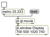
This shows a simple way to play a QuickTime movie using Jitter. When the jit.qt.movie object receives a read message, it opens a dialog box allowing you to select a movie file. As soon as you select a movie and click OK, jit.qt.movie begins to retrieve frames of video from that file and place them in memory, at the frames-per-second rate specified in the movie file itself. (It also begins playing the audio soundtrack of the video.) But for you to see the video, you need to create a window in which to display it, and you need to tell that window what to display. The jit.window object creates a window, with whatever name you give it in the first argument, at the location you specify in the next four arguments (the pixel offset coordinates of the left, top, right, and bottom edges of your window). Then, each time jit.qt.movie receives a bang it sends out information about the location of the image in memory, which the jit.window will refer to and draw. Because we expect that a video might have a frame rate as high as 30 frames per second, we use a metro to send a bang 30 times per second, i.e., every 33.333 ms. So,jit.qt.movie takes care of grabbing each frame of the video and putting it in memory, metro triggers it 30 times per second to convey that memory location to jit.window, and jit.window refers to that memory location and draws its contents.
January 20, 2011
Example 9: Attributes of jit.qt.movie.
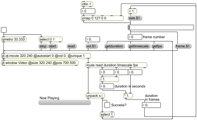
The jit.qt.movie object, for playing QuickTime videos, enacts many of the features made available by QuickTime, so it has a great many attributes and understands a great many messages. You can set some of its attributes with messages, such as its playback rate (with a rate message) or its audio volume (with a vol message). Some of its attributes are traits of the loaded movie file, and can't be altered (at least not without altering the contents of the movie file itself), such as its duration (the duration attribute). This patch shows how you can query jit.qt.movie for the state of its attributes, use that information to derive other information, and then use messages to tell jit.qt.movie what to do, such as using a frame message to tell jit.qt.movie what frame of the video to go to.
January 25, 2011
lmap: Linear mapping equation.
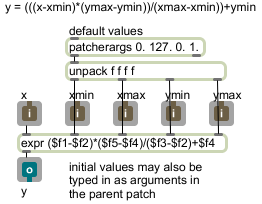
The term "mapping" refers to making a map of correspondences between a source domain and some other "target" range. (Think of the game where you are given words in one category and are challenged to try to find an appropriate correspondence in another category, as in "Kitten is to cat as puppy is to ...".) The simplest kind of numerical mapping is called "linear mapping". That's when a one-to-one correspondence is drawn from every value in a source range X to a value that holds an exactly comparable position in a target range Y. For example, in the target range 0 to 100, the value 20 holds exactly the same position as the value 2 does in the source range 0 to 10. In both cases, the value is 20% of the distance from the minimum to the maximum.
To convert one range into another linearly, there are really just two simple operations required: scaling (multiplication, to resize the range) and offsetting (addition, to push the range up or down). If you know the extent of two ranges X and Y, and a source value x, you can find the linearly corresponding target y value with this algebraic equation:
y = (((x-xmin)*(ymax-ymin))/(xmax-xmin))+ymin
This patch uses the expr object to implement that equation. In expr, the items such as $f1 and $f2 mean "the (floating point) number that has come in the first inlet", "the (floating point) number that has come in the second inlet", and so on. (Geeky technical note: We don't need to use quite as many parentheses in the expr object as we did in the equation above, because the ordering of mathematical operations is implicit, due to the operator precedence that is standard in almost all programming languages.)
This patch has inlet objects and an outlet object so that it can be used as an object in another patch. You just save this patch with the name "lmap" somewhere in Max's file search path, and you can then use it as a lmap object in any other patch. You establish the X and Y ranges by specifying their minimum and maximum (xmin, xmax, ymin, and ymax), then you send an x value in the left inlet to get the corresponding y value out the outlet. The patcherargs object supplies default initial values for xmin, xmax, ymin, and ymax in case no arguments are typed into the object when it's created in the parent patch; however, if values are typed in for xmin, xmax, ymin, and ymax (as in lmap 0. 1. -2. 2.), the patcherargs object inside lmap will send those values out instead of its default values.
Go ahead and download that patch and save it with the name "lmap", as it will be used in the next example. In Max, patches that are saved with a one-word filename and used as objects in another patch are called "abstractions". This lmap abstraction functions very much like the zmap object and scale object that already exist in Max, but I've provided lmap here so that you can see how one might implement the basic linear mapping function (in any language).
Example 10: Linear mapping and linear interpolation.
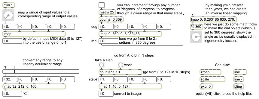
This patch shows examples of linear mapping and linear interpolation, using the lmap abstraction described above. One could substitute the built-in Max object scale in place of lmap with the same results.
As shown in the upper-left corner, with no arguments typed in lmap maps input values 0 to 127 (such as MIDI control data) into the range 0.0 to 1.0 (just as the scale object does by default). The output range 0.0 to 1.0 is useful for controlling the parameters of a lot of Jitter objects, and it's also a range that can be re-mapped to any other range with simple scaling and/or offsetting (multiplication and/or addition).
Just below that is a mundane example of how linear mapping applies to common everyday conversion, such as converting temperatures from Fahrenheit to Celcius.
You can use linear mapping to step through any range in a specific number of N steps, just by setting an input range from 1 to N and providing input x values that count from 1 to N. This is demonstrated by the part of the patch labeled "go from A to B in N steps". In effect, this is linear interpolation from A to B, since each step along the way will produce a corresponding intermediate value.
The part of the patch just above that demonstrates another case of the relationship between mapping and interpolation. The counter object counts cyclically in 360 steps from 0 to 359 (i.e., from 0 to almost 360), and we map the range 0 to 360 (the number of degrees in a circle) onto the output range 0 to 2π (the number of radians in a circle). Thus we're able to go continually from 0 to (almost) 2π by degrees. (We then map that value with an inverse relationship in order to cause the dial to show the radial angle changing counterclockwise as it would be graphed in Cartesian trigonometry. Setting ymin to be greater than ymax causes such an opposite mapping.)
The Max objects line, line~, and bline offer three methods for linear interpolation within a single object.
January 27, 2011
Example 11: Linear note movement.
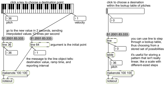
The line object interpolates linearly from its current value to some new destination value, ramping over a specified period of time, reporting its intermediate values along the way. In this example, we instruct line to ramp toward a given destination value, arriving there in 2 seconds, sending out a report of its progress (the intermediate values as it goes toward the destination) 12 times per second (i.e., once every 83.333 milliseconds). If you want line to do this sort of ramping behavior, you always need to give it a new destination time in its second inlet before you give it a destination value in its left inlet. Alternatively, you can give it all the information as a space-separated list of numbers, as is done here.
If you want to do a nonlinear mapping that you can't easily describe with an arithmetic formula, it's often best just to look up values in a stored array, also known as a "lookup table". You can describe a nonlinear function over time by stepping through the values in a table. In the left inlet you specify the location that you want to access within the table (with location indices numbered starting at 0), and table sends out the value that's stored at that location. In this example, we stored a synthetic musical scale in the table. (Double-click on the table object to see a graph of its contents.) To store that information as part of the patch, you have to check the "Save Data With Patcher" option in the table's Inspector. Then, to play only notes that belong to that scale from cello low C (MIDI 36) to flute high C (MIDI 96), we just need to read through table indices 0 to 35.
Example 12: Random note choices.
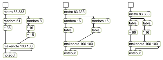
The left part of this example shows the use of the random object to make arbitrary note choices. Every time random receives a bang in its inlet, it sends out a randomly chosen number from 0 to one less than its argument. In this case it chooses one of 61 possible key numbers, sending out a number from 0 to 60. We then use a + object to offset that value by 36 semitones, transposing up three octaves to the range 36 to 96 -- cello low C to flute high C. Similarly, we choose one of 8 possible velocities for each note. The random object sends out a number from 0 to 7, which we scale by a factor of 16 and offset by 15, thus yielding 8 possible velocities from 15 to 127. These choices by the random objects are made completely arbitrarily (well, actually by a pseudo-random process that's too complex for us to detect any pattern), so the music sounds incomprehensible and aimless.
One can make random decisions with a little bit more musical "intelligence" by providing the computer with a little bit of musically biased information. Instead of choosing randomly from all possible notes of the keyboard, one can fill a table with a small number of desirable notes, and then choose randomly from among those. In the middle example, we have filled lookup tables with 16 possible velocity values and 16 possible pitches. Each time we want to play a note, we choose randomly from those tables. The velocities are mostly mezzo-forte, with only one possible forte value and one fortissimo value. Thus, we would expect that most notes would be mezzo-forte, with random accents occurring unpredictably on (on average!) one out of every eight notes. The pitches almost all belong to a Cm7 chord, with the exception of a single D and a single A in the upper register. So, statistically we would expect to hear a Cm7 sonority with an occasional 9th or 13th. There's no strong sense of melodic organization, because each note choice is made by random with no regard for any previous or future choices, but the limited, biased set of possibilities lends more musical coherence to the results.
In a completely different usage of the table object, you can use table as a probability distribution table, by sending it bang messages instead of index numbers. When table receives a bang, it treats its stored values as relative probabilities, and sends out a chosen index number (not the value stored at that index) with a likelihood that corresponds to the stored probability at that index. Double-click on the table objects in the right part of the patch to see the probabilities that are stored there. In the velocity table, you can see that there is a relatively high probability of sending out index numbers 4 or 5, and a much lesser likelihood of sending out index numbers 1 or 7. These output numbers then get multiplied by 16 to make a MIDI velocity value. Thus we would expect to hear mostly mezzo-forte notes (velocities 64 or 80) and only occasional soft or loud notes (velocities 16 or 112). In the pitch table, you can see that the index numbers with the highest probabilities are 0, 4, 7, and 11 respectively, with a very low likelihood of 2, 9, or 12. These values have 60 added them to transposed them to the middle octave of the keyboard. So we would expect to hear a Cmaj7 chord with only a very occasional D or A.
To learn more about the use of table to get weighted distributions of probabilities, read the blog article on "Probability distribution".
February 3, 2011
Example 13: Audio amplitude control.
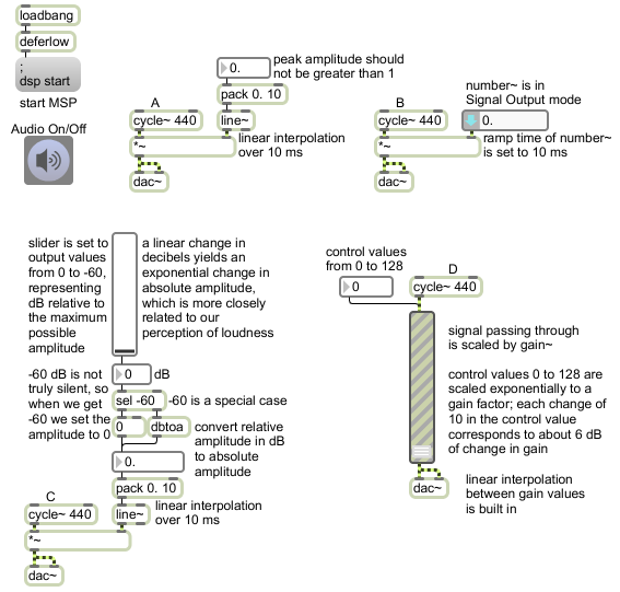
As explained in MSP Tutorial 2, in order to avoid creating clicks in audio when you change the amplitude, you need to interpolate smoothly from one gain value to another. Example A in this patch shows how to use the line~ object to do that. The gain value from the number box is combined with a transition time in the pack object (10 ms in this case) and the two numbers are sent as a list to line~. The line~ object interpolates to the new value sample-by-sample over the designated transition time (i.e. over the course of about 441 samples) to get to the destination gain value smoothly. Example B does exactly the same thing, but uses a single object, number~, to accomplish the same functionality as was achieved with number box, pack, and line~ in Example A. Note that the number~ object is in Signal Output mode (with the downward arrow on the left of the object), which enables it to function like a float number box and send out its value in the form of a signal (with a designated interpolation time).
To create a fade-in or fade-out that sounds linear to us perceptually, we actually have to do a fade that is exponential. Doing a linear fade in the decibel scale and then converting that value to an actual amplitude (gain) value is a good way to get a fade that sounds "right" (smooth and perceptually linear). The 16 bits of CD-quality digital audio theoretically provide up to 96 decibels of dynamic range, but in most real-world listening situations we probably only have 60 to 80 decibels of usable dynamic range above the ambient noise floor. Example C permits control of the amplitude of the signal in a range from 0 dB (full volume) down to -59 dB (very soft), and if the user chooses -60 dB with the slider (very soft but still not truly silent), we treat that as a special case by looking for it with the select -60 object, and turn the gain completely to 0 at that point.
The gain~ object in Example D combines the functionality of slider, exponential scaling (as with the scale object), line~, and *~. It's handy in that regard, because it takes care of lots of the math for you, but because its inner mathematics are not very intuitive to most users, you might find you have more precise control by building amplitude controls yourself in one of the ways shown in Examples A, B, and C.
For some very similar examples, with slightly different explanation, see also Example 12 from the previous year's class.
Example 14: Line segment control functions.
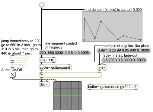
The line~ object is intended for use as a control signal for audio. You don't listen to line~ directly, but it's very effective as a controller/modifier/modulator of other signals. A pair of numbers (i.e. a two-item space-separated list of numbers) tells line~ a destination value and a time (in milliseconds) to get to that value. For example, the message 0.99 100 tells line~ to change its signal value from whatever it currently is to 0.99, moving linearly sample-by-sample toward 0.99 over the course of 100 milliseconds, calculating the intermediate signal value for each sample along the way. The result is a smoothly changing signal.
You can also send line~ a list that has more than two numbers. Every two numbers in the list are viewed as a "destination value / transition time" pair. The output of line~ follows the instructions of the first pair of numbers, then immediately follows the second pair, and so on. Thus, one can create a variety of control function shapes by specifying the destination value and transition time for each line segment.
In this patch, try clicking on the message box that says "example of a guitar-like pluck". The amplitude of the sound goes to full (0.99) in 1 millisecond, dies by -12 dB (to 0.25) in the next 99 milliseconds, dies another -14 dB (to 0.05) in the next 900 milliseconds, and then fades entirely to 0 in 3000 ms. The result is a 4-second note with roughly the amplitude envelope of a plucked string.
The message box just below that, labeled "fade-in, stay, fade-out", describes a very slow fade-in and fade-out. It goes to an amplitude of 0.5 in 2 seconds, stays there for 3 seconds, then fades to 0 in 5 seconds. The same sort of line segment function can also be used to control other aspects of a sound. The message box labeled "line segment control of frequency" specifies frequency values (to send a constantly changing frequency to cycle~) instead of amplitude values. It causes the frequency of the message box to jump immediately to 220 Hz, glide to 660 Hz in 3 seconds, shoot quickly down to 110 Hz in 5 milliseconds, then glide up to 440 Hz in about 7 seconds.
The function object allows you to draw a line segment function by clicking at the desired breakpoints. You can set the domain of that function (the total time of of the x axis) in the object's Inspector or with a setdomain message. In this example, we have set the function's domain to 10 seconds (10,000 ms). When the object receives a bang, it sends out its second outlet a list of destination value / transition time pairs that are designed to go to a line~ object, and that correspond to the shape of the drawn function. So, in this example we use one button to trigger the function to send a 10-second line segment function to the line~ that controls amplitude at the same time as we trigger the message box to send a 10-second function to the line~ that controls the frequency of the cycle~. The result is continuous modulation of the oscillator's frequency and its amplitude.
For more on the use of line segment control functions, see the chapters on the Algorithmic Composition blog, titled "Line-segment control function" and "Control function as a recognizable shape".
It's worth pointing out that the cycle~ object in this example uses 512 samples of a stored waveform in a buffer~ instead of its default cosine waveform. By giving a cycle~ object the same name as a buffer~, you instruct it to look at 512 samples of that buffer~ for its wavetable. The waveform being used in this example is one cycle of an electric guitar chord.
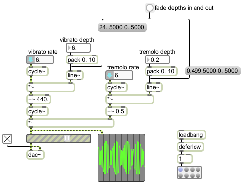
Example 15: Amplitude modulation and frequency modulation.
February 10, 2011
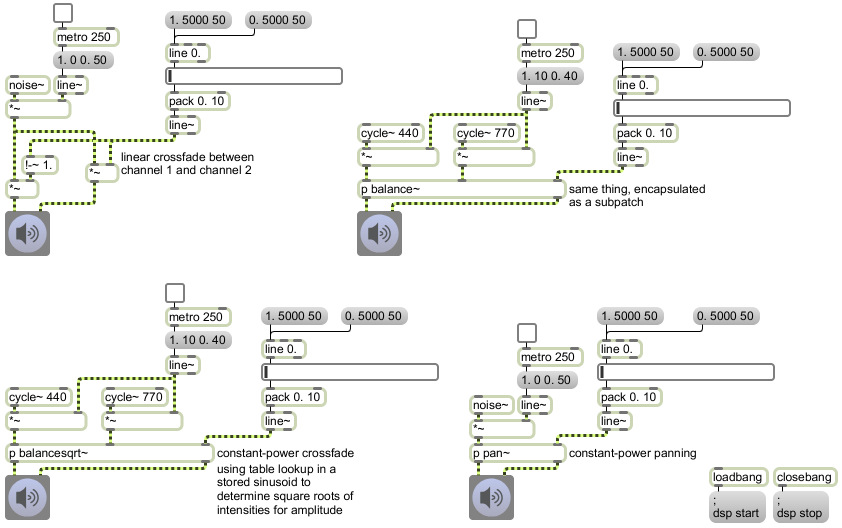
Example 16: Stereo balance and panning.
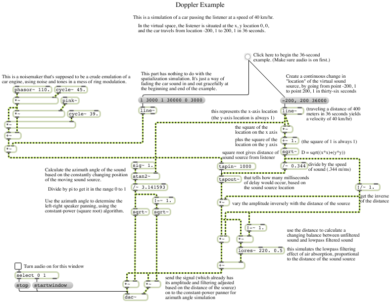
Example 17: Calculating doppler shift for moving virtual sound sources.
February 15, 2011
Example 18: Using gate to route messages.
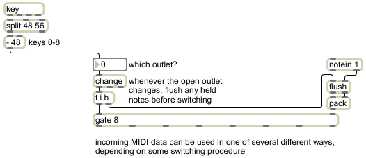
You can assign input data to have a different function at different times, simply by sending it to different parts of your program. For example, if you have a control device such as a MIDI keyboard or other MIDI controller with a limited number of keys, buttons, knobs, or faders, you can assign one control element to be the mode selector that changes the functionality of all the other elements. This program demonstrates one easy way to direct incoming MIDI note data to different destinations (where the data could have a different effect) using the gate object.
The argument to gate specifies how many outlets it should have. Messages that come in the right inlet are passed out the outlet specified by the most recent number received in the left inlet. (An optional second argument can specify which outlet should be open initially.) The outlets are numbered starting with 1. If the most recently received number in the left inlet is 0, or no open outlet has been specified, all outlets are closed.
In this patch, you can specify the open outlet via the number box, or by typing a number on the computer keyboard. Since the keys 0 to 9 on the keyboard have the ASCII values 48-57, it's easy to turn the ASCII values into the numbers 0 to 9 just by subtracting 48 from them. In the upper-left portion of the patch, we get the ASCII values with the key object, look only for ASCII values in the range 48 to 56 (keys 0 to 8), and subtract 48.
In the upper-right portion of the patch, we get MIDI note data (pitches and velocities) with the notein object, pass the pitches and velocities through a flush object, and pack them together as a two-item list with the pack object so that they can go into the right inlet of gate as a single message (thus keeping the pitch and velocity linked together).
Because the data that we're redirecting with gate is MIDI note data it's important that we not switch outlets while a MIDI note is being held, because that would likely result in a stuck note (a note-on message without a corresponding note-off message) somewhere in the program. For that reason, each time that we detect a change in the specified outlet number (with the change object), we first send a bang to the left inlet of flush, which causes it to sent out note-off messages for each held note-on, before we pass the new outlet number to the left inlet of gate. That ensures that the note-off messages go out the previously open outlet before we switch to a new outlet for subsequent notes. (This practice of making sure you neatly close down one process when switching to another is a good habit to develop in your programming.)
pinger: a beeping test sound.
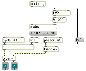
This patch is designed to be used as an abstraction (subpatch) in the next example. In order for the next example to work, you should download this example and save it with the filename "pinger.maxpat" somewhere in the Max file search path.
Its purpose is just to generate a recognizable sound. It emits very short sinusoidal beeps of a specified frequency, at a rate of a specified number of beeps per second, panning back and forth from left to right a specified number of times per second. These three parameters -- tone frequency, note rate, and panning rate -- are specified as arguments 1, 2, and 3 in the parent patch.
Because this abstraction was designed just to be used as a test tone in a particular example, it just uses the simple #1, #2, and #3 arguments as a way of providing the parameter values (as unchangeable constants typed in the parent patch). To make a more versatile program, one could also provide inlets to receive variable values, and could use patcherargs to provide useful default initial values. Compare, for example, the lmap abstraction presented on January 25, 2011.
Example 19: Mixing multiple audio processes.
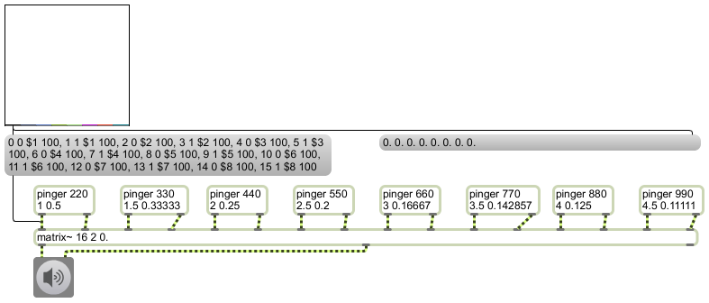
For this example to work correctly you will need to first download the pinger abstraction and save it with the filename "pinger.maxpat" somewhere in the Max file search path.
This example shows the use of the matrix~ object to mix together different sounds. Think of matrix~ as an audio mixer/router (a kind of combination of mixer and patch bay). The first two arguments specify the number of inlets and outlets, and the third argument specifies the default gain factor for each inlet-outlet connection.
Inlets and outlets of matrix~ are numbered starting from 0. So, in this example there are 16 inlets (numbered 0 to 15) and 2 outlets (numbered 0 to 1). (There's always an extra outlet on the right, from which informational messages are sometimes sent.)
Messages to the left inlet of matrix~ generally take the form of a four-item list to specify an inlet, an outlet to be connected that inlet, a gain factor (multiplier) for sounds that will flow from that inlet to that outlet, and a ramp time to transition smoothly to that gain factor (to avoid clicks). You can send as many such messages as you'd like, to specify as many connections as you want.
In this example we have connected eight stereo pinger objects to the 16 inlets of matrix~, and we will mix them all together for a single stereo output. The pinger objects are just stand-ins for what could potentially be any eight different audio processes you might want to mix together. The arguments to pinger specify frequency of the beep tone, the number of notes per second, and the rate of panning. For example, the first pinger plays a 220 Hz tone 1 time per second (i.e., at a rate of 1 Hz), panning left to right once every two seconds (i.e. at a rate of 0.5 Hz). The next pinger plays a 330 Hz tone at a rate of 1.5 notes per second (i.e. once every 666.6667 milliseconds), panning left to right once every three seconds (i.e., at a rate of 0.33333 Hz), and so on. The result is 8 tones (harmonics 2 through 9 of the fundamental frequency of 110 Hz) at 8 different harmonically-related rhythmic rates, panning back and forth at 8 different harmonically-related rhythmic rates.
With matrix~ you can mix these eight tones in any proportion you want, but how can you easily control all eight amplitudes at once? If you had a MIDI fader box, you could map the eight control values from the faders to the gain factors of the various connections. In the absence of such a fader box, we use the multislider object, set to have 8 sliders, that sends out a list of eight values from 0. to 1. corresponding to the vertical position of each slider as drawn with the mouse. So, by clicking and/or dragging with the mouse on the multislider you can set eight level values for use by matrix~. That list of eight values is sent to the right inlet of the right message box so we can see the values, and it's also sent to the left inlet of the left message box where the values are used in sixteen different connection messages to matrix~.
Take a moment to examine and understand those messages. The first message says "connect the first inlet [inlet 0] to the first outlet [outlet 0] multiplied by a gain factor [the value of the first slider] with a transition time of 100 milliseconds, and so on. Each pair of messages controls a pair of inlets corresponding to one of the pingers, and sets the gain with which that pinger will go to the output.
Turn on audio audio by clicking on the ezdac~, then try out the patch by moving the sliders in the multislider. Note that when you add together eight different audio processes, each playing at full volume, you need to be careful about the sum of all your gain factors. A more elaborate patch would, at the least, provide a volume control for the final summed signal. Even more desirably, perhaps, the final volume control could be constantly controlled automatically, proportionally to the sum of the slider values, to prevent clipping of the output signal.
March 3, 2011
Example 20: Windowing an audio signal.
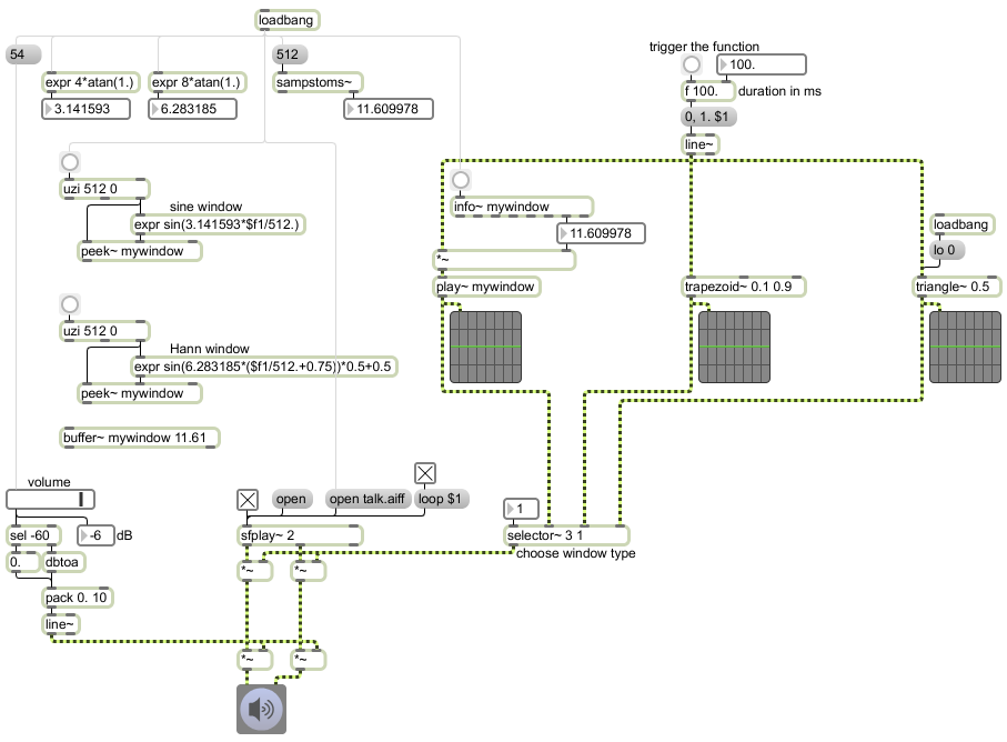
In signal processing, a "window" is a function (shape) that is nonzero for some period of time, and zero before and after that period. When multiplied by another signal, it produces an output of 0 except during the nonzero portion of the window, when it exposes the other signal. The simplest example is a rectangular window, which is 0, then briefly is 1, then reverts to 0. The windowed signal will be audible only when it is being multiplied by 1 -- i.e., during the time when the rectangular windowing occurs. Many other window shapes are possible: trapezoidal, triangular, a "sine" window (the first half of a sine wave), etc.
Windowing is most often used in spectral analysis, to view a short time segment of a longer signal and analyze its frequency content. Windows are also used to create short sound segments of a few milliseconds' duration called "grains", which can be combined into granular sound clouds for unique sorts of synthesis. In general, one can think of any finite sound that has a starting point and a stopping point as being a windowed segment in time. For example, a cycle~ object is always producing a signal, but we can window it with a *~ object, keeping its amplitude at 0 except when we want to hear it. However, a rectangular window -- suddenly switching from 0 to 1 and then back from 1 to 0 -- will usually create a click, so other window shapes are usually more desirable.
This patch shows several ways to create a window function in MSP. To read through the function, you need some sort of linear signal such as line~, phasor~, count~, or the right outlet of groove~. The MSP objects trapezoid~ and triangle can convert a linear 0-to-1 signal into various sorts of trapezoidal or triangular functions. You can also use a math expression to calculate some other function arithmetically; you can either do that on the fly or, more economically, do it in advance, store the result in a memory buffer, then read through the buffer whenever you need that window shape. That last method is what's being done with the buffer~, peek~, and play~ objects.
In the top left part of the patch, we see some ways to obtain useful constants for mathematical computations. For example, pi and 2pi are numbers that are often needed for computing a cyclic waveform (or a part of one). Once you know the constant value you need, you can plug it into your own math expression. The sampstoms~ object is useful for figuring out how many milliseconds correspond to a certain number of audio samples. (And the reverse calculation can be made using its counterpart mstosamps~.) In this case, we learn that 512 samples at a sampling rate of 44,1000 Hz is equal to 11.61 milliseconds, so we create a buffer~ of exactly that length. Then we use uzi, expr, and peek~ to quickly fill that buffer with 512 samples describing half of a sine wave, which will be our window shape. (Double-click on the buffer~ to see its contents.) The formula for another common window shape, known as a Hann window, is also shown just below that.
Then, you can play a sound file with sfplay~, choose one of the three window functions with the selector~ (the sine window is initially chosen by default), and trigger a window to occur by clicking on the button at the top of the patch.
This sort of windowing technique is useful for shaping the amplitude envelope of sampled sounds or any other audio signals, in order to avoid clicks and to create the sort of attack and release characteristics you want for a sound, whether it be a short grain or a longer excerpt.
Example 21: Rhythmic delays in time with a musical tempo.
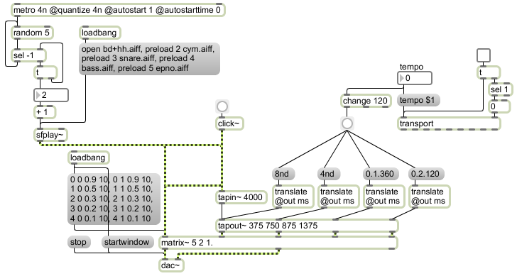
The tempo-relative timing capabilities in Max can be used to synchronize MSP processing in time with a musical beat. In this example, timings of delays are specified in tempo-relative time units so that they remain rhythmically correct for any tempo.
Click on the button above the click~ and you will hear a click followed by four rhythmically delayed versions of the click (with diminishing amplitudes). The timings of the delays have been set to a dotted eighth note, a dotted quarter note, a double-dotted quarter note, and a half-note-plus-a-sixteenth. The tapout~ object does not interpret tempo-relative time syntax on its own, so we use the translate object to convert time musical units such as 8nd or bars.beats.units such as 0.1.360 into milliseconds.
Now try changing the tempo of the transport to some other tempo such as 96 bpm, and then trigger the click again. Notice how the rate of the rhythm has changed commensurate with the change in the global tempo. Finally, start the transport, which will also start the metro, which will begin playing a different sound every quarter note. Since the delays are all set to happen on sixteenth note pulses somewhere between the quarter notes, you will hear a composite rhythm that is more complex than is actually being played by the metro. If you change the tempo, the delays will stay in the same rhythmic relationship to the quarter-note beat.
March 8, 2011
Example 22: Routing MIDI to other applications.
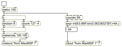
The easiest way to establish MIDI connection between Max and other applications on the same computer is via the "virtual" MIDI ports Max provides. Max creates two virtual input ports and two virtual output ports that can be accessed by other MIDI applications. (You can see those virtual ports listed in Max's MIDI Setup, by choosing MIDI Setup... from the Options menu.)
This example shows how one can generate MIDI information in Max and send it to another application. Here note information and controller information is being sent to the virtual port "from MaxMSP 1". Any application that's set to receive MIDI input from that virtual port will get the data that Max is transmitting. In this case Max is generating a cloud of random notes and is also moving the volume up and down in a sinusoidal fashion every 100 notes.
Example 23: MIDI and audio via ReWire.
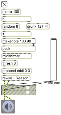
Max can interface with other applications via ReWire. Max can act as either a ReWire host or a ReWire client. Max can be a client to an open host application just by choosing "ad_rewire" as the MSP audio driver in the DSP Status window. Alternatively, you can use Max as the host (mixer) application by including the rewire~ object in your program. This establishes Max as a mixer (host) application, and a ReWire-capable synth application that you open while Max is a mixer will pipe its audio to MSP via the outlets of the rewire~ object.
This example shows Max in use as a host to the synth program Reason. Max can send formatted MIDI messages to Reason to play notes and control parameters of the Reason devices (see the rewire~ reference page for details), and MSP can further process the synth audio after it comes out of rewire~. Here Max is generating note information, formatting it as MIDI messages and sending those to the rewire~ object to be transmitted to Reason via ReWire. The audio that Reason produces in response will be piped back to Max via ReWire, where it can be used in MSP. (In this case MSP is only being used to control the output volume, but the sound received via ReWire can be treated just like any other MSP audio signal.)
Example 24: TouchOSC data via wireless UDP.
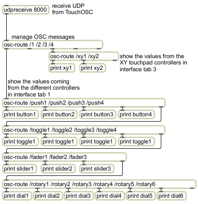
You can send messages to Max wirelessly from a mobile device such as iPhone, iPod Touch, iPad, or Android-based smart phone or tablet, using the TouchOSC app. You can read more about the OSC communication protocol that is used by TouchOSC, and you can download Max objects for managing OSC messages as part of the package of useful Max objects distributed freely by CNMAT at UC Berkeley. (You will need the CNMAT Max external object osc-route in order for this example patch to work.)
This patch uses the udpreceive object to receive wireless UDP data from a device transmitting on virtual port 8000. It uses the CNMAT Max external object osc-route to parse the OSC messages coming from TouchOSC. This patch has been set up to work with the TouchOSC default interface "Mix 2". It will print all the data coming from tabs 1 and 3 in the "Mix 2" TouchOSC interface. The first part of the OSC message indicates the tab number (such as /1), and the next part of the message indicates the interface object that sent the message (such as /fader1), and the last part of the message is the useful data from that object.
This program can receive WiFi data via a local network that you create on your own computer, or via the Internet.
This page was last modified March 13, 2011.
Christopher Dobrian
dobrian@uci.edu