Example 1: Open a sound file and play it.
This page contains links to explanations and example Max patches that are intended to give instruction on some basic concepts of interactive arts programming using Max.
The examples were written for use by students in the Interactive Arts Programming and Music Technology courses at UCI, and are made available on the WWW for all interested Max/MSP/Jitter users and instructors. If you use the text or examples provided here, please give due credit to the author, Christopher Dobrian.
There are also some examples from the previous years' classes available on the Web: examples from 2011's winter quarter Music Technology seminar, examples from 2010's Interactive Arts Programming class, examples from 2009's class, examples from 2007's class, examples from 2006's class, examples from 2005's class, and MSP examples and Jitter examples from 2004's class.
While not specifically intended to teach Max programming, each chapter of Christopher Dobrian's algorithmic composition blog contains a Max program demonstrating the chapter's topic, many of which address fundamental concepts in programming algorithmic music and media composition.
You can find even more MSP examples on the professor's 2007 web page for Music 147: Computer Audio and Music Programming.
And you can find still more Max/MSP/Jitter examples from the Summer 2005 COSMOS course on "Computer Music and Computer Graphics".
Please note that all the examples from the years prior to 2009 are designed for versions of Max prior to Max 5, and the examples from 2010 and 2011 are designed for Max 5. Therefore, when opened in Max 6 they may not appear quite as they were originally designed (and as they are depicted), and they may employ some techniques that seem antiquated or obsolete due to new features introduced in Max 6. However, they should all still work correctly.
[Each image below is linked to a file of JSON code containing the actual Max patch.
Right-click on an image to download the .maxpat file directly to disk, which you can then open in Max.]
Examples will be added after each class session.
January 12, 2012
Example 1: Open a sound file and play it.
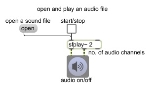
This shows an extremely bare-bones program for audio file playback.
1. Click on the speaker button (ezdac~ object) to turn audio on.
2. Click on the word "open" (message object) to open a dialog box that allows you to select a sound file. (In the dialog, select a WAVE or AIFF file and click Open.)
3. Click on the toggle object to start and stop playing. (The toggle alternately sends a "1" or "0" to the sfplay~ object, which sfplay~ interprets as "start" and "stop".)
The sfplay~ box is an MSP object. It performs an audio task: it plays sound files from disk and sends the audio signal out its outlets. The number 2 after sfplay~ is an 'argument', giving the object some additional information: that it should play in stereo, and thus should have two audio signal outlets. (The third outlet will send a notifying message when the soundfile is done playing, but this program doesn't use that outlet.) The speaker button (a.k.a. the ezdac~ object) is a 'user interface object'. It allows the user to interact with the program (in this case, by clicking on it with a mouse) and it performs a task (to turn audio on and off, and to play whatever audio signals it receives in its inlets as long as audio is turned on). Notice that the patch cords between the outlets of sfplay~ and ezdac~ are yellow and striped; that indicates that what is being passed between those objects is audio signal. The open object is a 'message box'. It's a user interface object, too. When clicked upon, it sends the message it contains (in this case, the word 'open') out the outlet to some other object. This is a message that sfplay~ understands. (If it were not, sfplay~ would print an error message in the Max window when it received an unfamiliar message.) The plain black patch cord indicates that what is passed between these objects is a single message that happens at a specific instant in time rather than an ongoing stream of audio data. The words 'start/stop' and 'audio on/off' are called comments. They don't do anything. They're just labels to give some information.
Here are a few thoughts for you to investigate on your own.
If you wanted audio to be turned on automatically when the patch is opened, and/or the 'Open File' dialog box to be opened automatically, how would you make that happen? (Hint: See loadbang.)
If you want to cause something to happen when the file is done playing, how would you do that? (Hint: Read about the right outlet of sfplay~.)
If you wanted to play the file at a different speed than the original, how would you do that? (Hint: Read about the right inlet of sfplay~.)
A single sfplay~ object can only play one sound file at a time, but it can actually access a choice of several preloaded sound files. How can you make it do that? (Hint: Read about the preload message to sfplay~.)
Suppose you'd like to be able just to pause sfplay~ and then have it resume playing from the spot where it left off rather than start from the beginning of the sound file again. Is that possible? (Hint: Read about the pause and resume messages to splay~.)
What if you want to start playback from the computer keyboard instead of with the mouse? (Hint: See key -- and/or keyup -- and select.)
Suppose you want to have control over the loudness of the file playback. What mathematical operation corresponds to amplification (gain control)? (Hint: See *~. See also gain~.)
January 17, 2012
Example 2: Using Presentation Mode
This program demonstrates how objects in Presentation Mode can have a different location and appearance than they do in Patching Mode. Select the objects that you want to have appear in the presentation, and choose the Add To Presentation command from the Object menu. Then, to switch to Presentation Mode, click on the small easel icon at the bottom of the window (or type command-option-E). Now you see only the objects that will appear in the Presentation. While in Presentation Mode (but still in "unlocked" Edit mode) you can move those objects, resize them, and change their appearance attributes in their Inspector. To force your patch to open in Presentation Mode, choose the Patcher Inspector command from the View menu (or type command-shift-I), and check the "Open In Presentation" option.
This file has been saved to open in Presentation mode. To see the working patch behind the scenes, type command-option-E to go from Presentation Mode to Patching Mode, then type command-E to go from Locked (Running) Mode to Unlocked (Edit) Mode, and expand the window to see the whole patch (which looks like the graphic above.
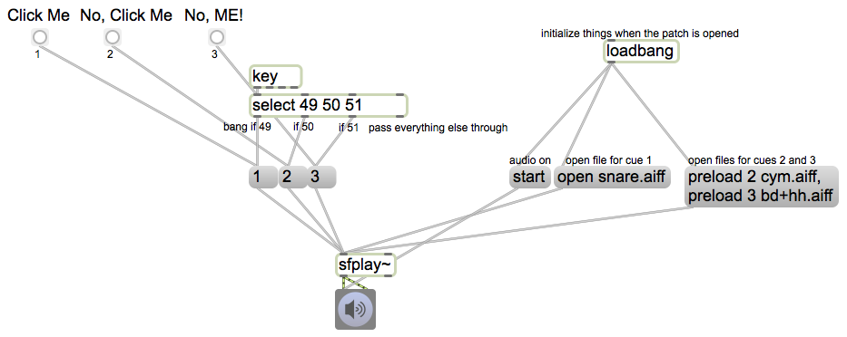
This patch uses the loadbang object to set up the desired initial conditions: it opens three audio files, then turns audio on, so it's ready to play the files. The 'open' message to sfplay~ is used to designate a file for cue number 1. Any other numbered cues must be designated by the 'preload' message (followed by the desired cue number and then the file name). These three numbered cue messages '1', '2', and '3' are triggered either by the three buttons or by the "1", "2", and "3" keys on the computer keyboard (ASCII codes 49, 50, and 51). The select object detects those three ASCII codes.
So the program just allows you to trigger one of three soundfiles, either by clicking on buttons or typing on keys. It demonstrates the use of the loadbang object to intialize conditions, the select object to detect specific key presses, and the use of Presentation Mode to present to the user the exact interface you want him/her to see.
January 19, 2012
Example 3: Line segment control functions
In some past examples (e.g., Example 5 from 2011) you can see how the line~ object interpolates sample-by-sample in a straight line from one value to another. You provide it with a pair of numbers -- a destination value to go to, and an amount of time in which to get there -- and it changes gradually (linearly) to that destination value in that amount of time.
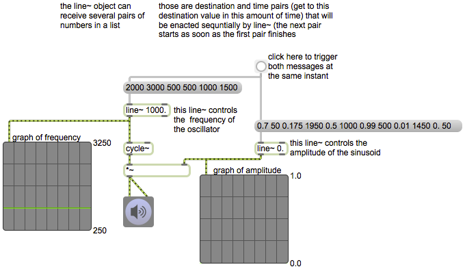
This example shows that you can actually provide line~ with a longer list of numbers, and it will break the list up into pairs of numbers -- each pair representing a destination value and a ramp time -- and will enact each pair one after the other. This results in a control shape that's made up of a series of line segments instead of a single straight line.
You can make a large variety of shapes with various lists. In this example we just use two shapes: one for the frequency of an oscillator and another for that oscillator's amplitude. (Notice that each of the two line~ objects has a typed-in argument specifying its initial value. When audio is first turned on, the oscillator's frequency is 1000 Hz and its amplitude is 0, because those are the signal values being provided by the line~ objects.) When you click on the button, you trigger both message boxes, sending the lists to the two line~ objects.
The frequency goes from 1000 Hz to 2000 Hz (one octave higher) in 3000 milliseconds (3 seconds), then drops two octaves to 500 Hz in 500 ms (1/2 second), then returns to 1000 Hz in 1500 ms. The amplitude fades quickly up to .7 in just 50 ms, then drops by -12 dB to 0.175 in 1950 ms, then goes up about 9 dB to 0.5 in 1000 ms (all that in the same amount of time that the frequency is going up one octave), then goes up another 6 dB to 0.99 in 500 ms, fades down about -40 dB to 0.01 in 1450 ms, and then goes completely to 0 in the last 50 ms. These two "envelopes" -- a frequency shape and an amplitude shape -- each take the same total amount of time (5 seconds) but are not identical. (N.B. Because the scope~ objects need to gather audio samples before drawing them, the visual display lags somewhat behind what you hear.)
January 24, 2012
Example 4: Two ways to get BPM timing
Sometimes its more convenient to think about musical time in "beats per minute" (BPM) instead of milliseconds. (Beats per minute is also a much better unit to use when you want to express an accelerando or decelerando.) Here are two easy ways to express timing in terms of beats per minute.
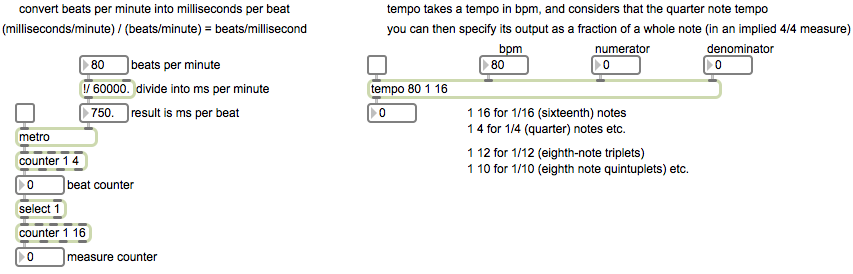
The metro object expects to receive its time interval in milliseconds. In order to cause metro to bang at a BPM rate, you just need to divide BPM (beats/minute) into 60000 (milliseconds/minute). The one-minute units cancel each other out, leaving a value in milliseconds per beat.
The patch on the right demonstrates the tempo object. It works rather like a combination of the metro and counter objects, but it uses BPM and metric divisions of a whole note to express the timing of its output. It assumes a whole note as one measure and a quarter note as one beat. You specify a tempo value in BPM, either as the first typed-in argument or as a number in the second inlet, and you specify a fraction to express the rhythmic values you want it to report. For example, the arguments 80 1 16 means "at a tempo of 80 quarter notes per minute, output every 1/16 note. It will output a count showing where it is in the 4/4 measure, starting at 0 and counting up to 15. (At a tempo of 80 BPM, one quarter note is 750 ms, so the interval between 16th-note pulses is 187.5 ms.)
Example 5: A 16-stage note sequencer
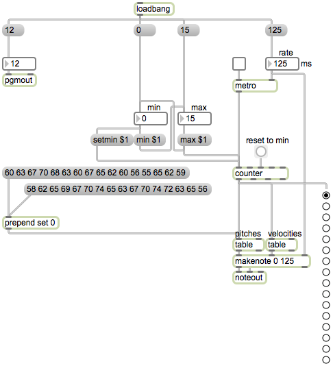
Analog synthesizers of the early 1970s often included a "sequencer" capable of cycling through a timed sequence of 16 different voltages (which would most commonly be used to control the pitch of an oscillator). This likely explains why so many fast 16-note repeating patterns appeared in electronic music of that time period. Most voltage sequencers allowed the user to set the voltage for each step of the sequence, and to adjust the timing interval (rate) of the sequence. This patch imitates those sequencers, using MIDI pitches instead of a voltage-controlled oscillator.
The MIDI pitches and velocities of the sequence are stored in table objects (arrays), one for the pitches and one for the velocities. The table objects are set (in their Inspector) to "Save Data with Patcher", so they already contain a pattern of pitches and velocities when the patch is opened. You can play the sequence by turning on the metro, and you can change the speed of the sequence by changing the rate of the metro.
You can change the contents of a table by sending it a 'set' message. The first argument of 'set' is the index where you want to start saving values, and the subsequent numbers will be stored beginning at that index. So, in this example, when you click on one of the message boxes that contains a list of pitches, it gets the words "set 0" placed before it (indicating to set values of the table, starting at index 0) and thus replaces the contents of the pitch table.
Some sequencers (notably on Buchla synthesizers of that period) allowed the user to change the starting and ending stage of the sequence. In this patch we use number boxes to set the minimum and maximum output of the counter object, causing it to cycle through specific numbers within the 0-15 range. (Note that we also use the output of the "min" and "max" number boxes to set each other's minimum and maximum values, so that the minimum will always be less than or equal to the maximum.)
The visual display object on the lower right is a radiogroup object. It's normally used as a user interface object that allows a user to choose one of several items, but in this case we're just using it as a handy way to display which stage of the sequence is currently playing.
Turn on the metro, experiment with different rates, change the pitch content, and experiment with different "min" and "max" limits for the counter.
January 26, 2012
Example 6: Movie attributes
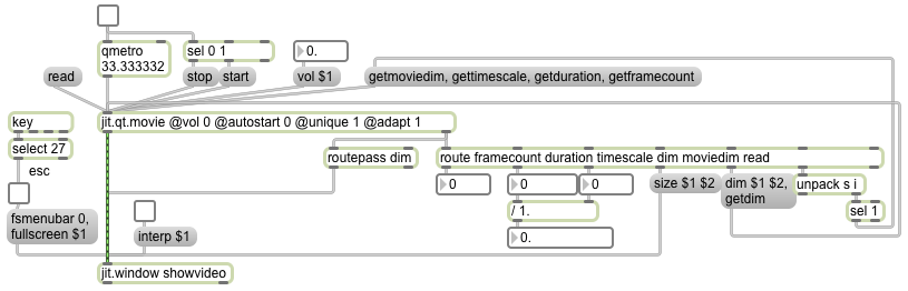
The jit.qt.movie object has a large number of attributes that you can use either to modify the object's behavior or to get information about the video it's playing. To set an attribute, you send a message consisting of the name of the attribute followed by the value(s) you want that attribute to have. For example, to set the 'vol' attribute (the volume of the video) to 0.5, you send the message 'vol 0.5' to jit.qt.movie. To find out what the value of a particular attribute is, just precede the attribute name with 'get', all in one word, such as 'getvol'. (Not all attributes are settable; some are only gettable.) When you request to get the state of an attribute (known as "querying" that attribute), the attribute name and value will come out the right outlet of jit.qt.movie (and most Jitter objects) as a single message, such as 'vol 0.5'. You can use the route object to look for particular types of messages by detecting the first word of the message (called the message's "selector" in object-oriented programming lingo). If route finds a match to one of its typed-in arguments, it will send the rest of the message (without the selector) out of its corresponding outlet.
You can also initialize the state of an object's attributes by typing in the attribute symbol '@' followed immediately (without a space) by the name of the attribute you want to set, followed (with a space) by the value of that attribute. In this example, the jit.qt.movie object has four of its attributes initialized to something other than their normal default values. The vol attribute is set to 0 (it's normally 1 by default) so that the audio will be silenced; the autostart attribute is set to 0 (it's normally 1 by default) so that the movie won't start to play automatically as soon as it's read in; the unique attribute is set to 1 (it's normally 0 by default) so that the object will only send out a jit_matrix message when it has a new frame of video that it hasn't previously sent (this means that even if it is triggered faster than its video's frame rate, it won't send out duplicate matrices); and the adapt attribute is set to 1 (it's normally 0 by default) meaning that the object will resize its internal matrix to be the right size for the movie it's trying to play.
Click on the read message box to open a video file. Here's a very handy fact: after jit.qt.movie tries to read in a video in response to a 'read' message, it sends out a read message of its own out the right outlet. The word 'read' is followed by the name of the movie file, followed by a 1 if the movie file was opened successfully or a 0 if the read was unsuccessful. By checking that success indicator, you can see whether the file was read in successfully, and if it was (i.e., if the sel 1 object sends out a bang), you can use that bang to trigger other things you might want to do. Here's what we decided to do...
As soon as the movie is opened successfully, we check its 'moviedim' attribute to learn its dimensions in pixels, we check the 'timescale' attribute to learn what QuickTime timing units it's using (how many time units per second it has, most commonly 600), we check the 'duration' attribute to see how long the movie is ('duration' is expressed in timescale units, which is why we need to know the timescale units first, so that we can calculate the duration in seconds), and we check the 'framecount' attribute to know how many frames are in the video. (So, although we don't do it in this example, you could divide the framecount, which is expressed in frames per second, by the duration in seconds, which you can calculate by dividing 'duration' by 'timescale', to learn the frames-per-second frame rate of the video. Or alternatively, you could query the 'fps' attribute, and use that to divide 'framecount' by 'fps' to learn the duration in seconds.)
If you look at the route object, you can see that we're using it to detect the different messages that will come out. It detects the 'read' message to know whether the movie has opened successfully, it detects the 'moviedim' message to learn the movie's dimensions and sends that information back to jit.qt.movie as part of a 'dim' message to resize the object's internal matrix and also sends it to jit.window as part of a 'size' message to resize the display window, it uses the timescale and duration information to calculate the movie's duration in seconds, and it shows us how many frames total are in the video.
The 'interp 1' or 'interp 0' message to jit.window will turn interpolation on or off. If the user resizes the display window to enlarge it (by dragging on the lower right corner of it), the window will be larger than the dimensions of the matrix it's receiving, and the video may appear somewhat "pixelated" and blocky. Turning interpolation on causes jit.window to interpolated between pixels instead of simply duplicating pixels, which will make the video appear less jaggedly pixelated.
If you want to fill the entire screen with the contents of jit.window, you can send the message 'fullscreen 1' to jit.window to turn on its 'fullscreen' attribute. If you also want to hide the menubar when it goes to fullscreen, you can set the 'fsmenubar' attribute to 0 (meaning "no menubar when going to fullscreen"). HOWEVER, beware. If you fill the screen and hide the menubar, how will you ever get back to your Max patch? It's a good idea, before you send any of those messages, to give yourself a way to toggle 'fullscreen' on and off. In this patch, we use the escape key (ASCII code 27) to bang a toggle so that we can switch back and forth between 'fullscreen 1' and 'fullscreen 0' without needing to use the mouse.
Example 7: simplest possible A-B video switcher
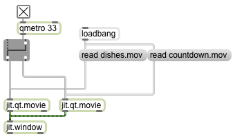
This is the simplest possible way to switch between two videos. When the patch is opened we read in a couple of example video clips (which reside in ./patches/media/ within the Max application folder, so they should normally be in the file search path). Because the default state of the 'autostart' attribute in jit.qt.movie is 1, the movies start playing immediately. Because the default state of the 'loop' attribute in jit.qt.movie is 1, the movies will loop continually. Click on the toggle to start the qmetro; the bangs from the qmetro will go out one outlet of the ggate (the outlet being pointed to by the graphic), and will thus go to one of the two jit.qt.movie objects and display that movie. Click on the ggate to toggle its output to the other outlet; now the bangs from the qmetro are routed to the other jit.qt.movie object, so we see that movie instead. (Note: You can also send a bang in the left inet of ggate to toggle it back and forth, or you can send it the messages 0 and 1 to specify left or right outlet.)
If you don't know the difference between a metro object and a qmetro object, you can read about it in this page on "Event Priority in Max (Scheduler vs. Queue)". In short, qmetro is exactly like metro except that it runs at a lower level of priority in Max's scheduler; when Max's "Overdrive" option is checked, Max will prioritize timing events triggered by metro over those triggered by qmetro. Since the precise timing of a video frame's appearance is less crucial than the precise timing of an audio or musical event (we don't notice usually when a frame of video appears a fraction of a second late or even occasionally is missing altogether, but we do notice when audio drops out or when a musical event is late), it makes sense to trigger video display with the low-priority scheduler most of the time.
Example 8: A-B video switcher
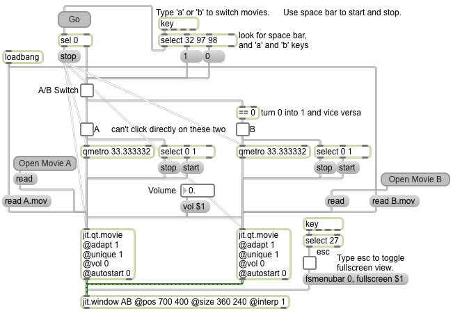
This is a more refined sort of A-B video switcher patch than the simple one shown in Example 7 above. It has a considerably more sophisticated user interface when viewed in Presentation mode. It will try to open two video files called "A.mov" and "B.mov", and it also provides buttons for the user to open any other videos to use as the A and B rolls.
Another possibly significant difference is that in this example we stop the movie that is not being viewed, and then when we switch back to that movie we restart it from the place it left off. In the previous example both movies were running all the time. If you need for the two movies always to be synchronized, you can either leave them both running as in the previous example, OR, whenever you stop one jit.qt.movie object, you can get its current 'time' attribute value and use that value to set the 'time' attribute of the other jit.qt.movie object when you start that one. (That's not demonstrated in this example.)
Example 9: stop-action slideshow (backward)
.png)
Here's an example of algorithmic video editing in Jitter. The goal is to create a stop action slideshow of single frames of video, stepping through a video in 1-second increments. And just to make it a bit weirder and more challenging, we'll step through the movie backward, from end to beginning.
Some information we might need to know in order to do this properly is the frame rate (frames per second) of the video so that we know how many frames to move ahead or backward in order to move one second's worth of time. We might also want to know the total number of frames in the video, so we know where to begin and end. Finally, we need to make a decision about how quickly we want to step through the "slideshow". In this example, by default we step through it one second at a time, but we make this rate adjustable with a number box.
When you read in a movie (it should be at least several seconds long, since we're going to be leaping through it in 1-second increments) jit.qt.movie sends out a 'read' message reporting whether it read the movie file successfully. If it did, we request information about the frames per second (fps) and number of frames (framecount), information that's contained in the movie file itself, and that jit.qt.movie can provide for us. We use that information to calculate the duration of the movie in seconds (framecount/fps), and to set the step size and limit of our stepping calculations.
The slideshow step calculator works like this. Starting at frame 0, use the + object to add one second's worth of frames to move ahead one second, use the % (modulo) object to keep the numbers within the range of total frames in the video (% is most useful for keeping numbers cycling within a given range), and then (because we actually want to be moving backward rather than forward) we subtract the frame number from the total number of frames in the !- object. (You could omit that object if you wanted your slideshow to move forward.) We send that resulting frame number to jit.qt.movie as part of a 'frame' message to cause it to go to that frame, and then we send a bang right after that to cause it to send its matrix information to jit.window. Also, we send the original number (before the !- object) to a pipe object to delay it a certain number of milliseconds, then it goes right back into the i object at the top to start the process over. (This will go on endlessly until pipe receives a 'stop' message that causes it to cancel its scheduled next output.)
January 31, 2012
Example 10: Linear mapping of ranges
To translate numbers that occupy a particular range into an equivalent set of numbers in a different range, one common and useful technique is "linear mapping". The term "mapping" refers to making conceptual connections between elements of one domain and elements of another, and "linear" mapping refers to using a mapping function that is a straight line--that is, such that numbers in one domain are mapped to an exactly equivalent position in the new domain. This is a very common and useful operation in media programming.
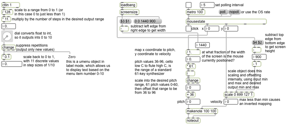
To do such a mapping requires the following operations. First, scale the range of the input values to occupy the desired range of outputs. The scaling operation is done by multiplication. An example of this would be if you want to map numbers that range from 0 to 127 (128 discrete integer values) into the range from 0 to 1); you could simply multiply all the input values by 1/127 (i.e., 1/(maximum-minimum) of the input range), which would result in outputs ranging from 0 to 1 in increments of 1/127, i.e., steps of size 0.007874. Then, if the entire output range needs to be adjusted upward or downward, you can offset the output by a certain amount. The offsetting operation is done by addition.
When the input range is divided up into a specific number of possible values, as is the case with integers 0 to 127 where there are 128 discrete possibilities, you might in some cases want to change the number of steps in the output range. In the example above, we had 128 discrete input values and wanted to map that onto the output range 0 to 1; but suppose we wanted the output to be only one of 11 discrete values, from 0 to 1 in increments of 1/10 (0.0, 0.1, 0.2, 0.3, ... 1.0). We can multiply by the desired number of output values by 11 (the desired number of possible outputs) and divide by 128 (the number of possible inputs), convert those values to integers (by truncating the fractional part of the number), then scale that new range to the desired range by the method described in the previous paragraph (and finally adding an offset if necessary).
That's what we did in the example on the left side of the patch. We take MIDI controller values from the mod wheel of a synthesizer (controller number 1, with 128 possible data values from 0 to 127), divide by 128 (the total number of possible inputs), multiply by 11 (the number of steps we want in our output range), convert the numbers to integers (the dial object does that for us internally by changing the data type from float to int), filtering out repetitions (the change object does that), resulting in 11 possible output values 0 to 10. To scale the range 0-10 down to the range 0-1, we multiply by 1/(maximum-minimum), which is to say 1/(10-0), which is 1/10, which is 0.1. That gives us 11 possible numbers ranging from 0 to 1 in ten equal steps.
Optionally you could re-scale that to any other size range (for example, multiply it by 100, which would give you a range from 0 to 100 in ten equal steps) and/or offset it by some amount. (for example, after multiplying by 100 you could add -50, which would give you a range from -50 to 50 in ten steps, i.e., -50, -40, -30, ... 50).
On the right side of the patch, we use the cursor (mouse) coordinates on the screen to control the pitch and velocity of MIDI notes. First we get the dimensions of the screen, using the screensize object. It outputs the left, top, right, and bottom coordinates of the screen. By subtracting left from right, and top from bottom, we obtain the width and height of the screen, in pixels. Those are our input ranges. We convert the horizontal range into 61 discrete steps from 0 to 60, filter out repetitions, then offset that range by 36 to get an output range of 36-96. Those will be our pitch values for MIDI notes, chosen based on the horizontal position of the cursor. For velocities, we use the vertical coordinate of the cursor within the total range of pixel possibilities, mapped into the range 1 to 127 to determine the note's velocity. The scale object actually does all the scaling and offsetting for us internally; all we have to do is specify the minimum and maximum values of the input range, and the minimum and maximum values of the desired output range. Notice one interesting wrinkle: because we want the velocity to decrease as the y pixel value increases, we give scale an output range with the minimum and maximum reversed, which results in an inverted linear mapping.
You can see this mathematical procedure of linear mapping encapsulated as an abstraction in this linear mapping equation example from last year's class, and you can see it in action in this linear mapping and linear interpolation example.
February 2, 2012
Example 11: Tempo-relative timing with the transport object
This patch doesn't do anything musical in its own right, but it shows some features of the transport object for tempo-relative control of timing in Max. For several other examples online of how to implement tempo-relative timing in Max, see Examples 42 through 48 from the 2010 IAP class.
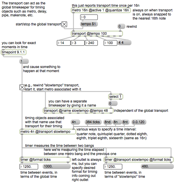
The transport object controls a global beat-based clock running at a specific metronomic tempo expressed in beats per minute (bpm). Other timing objects such as metro, delay, pipe, makenote, etc. can be synchronized to the global clock by specifying their timing interval in some tempo-relative format such as note values, ticks (parts per quarter note, usually 1/480 of a quarter note by default), or bars.beats.ticks.
At the top of this patch is a transport object for turning the global clock on and off. You can think of it like the tape-recorder-like controller that appears in most music sequencing software such as Pro Tools, Logic, Garage Band, Cubase, etc. You can set the global bpm tempo via the transport object's 'tempo' attribute, either with a typed-in attribute argument or by sending it a 'tempo' message. You can cause it to jump to a particular location in time by sending a point in time, expressed in ticks, in the right inlet. (So, for example, '0' causes it to rewind to the beginning of time.) Whenever it's running, other timing objects that have their timing units expressed in one of the tempo-relative timing formats will be controlled by the transport. So, when the transport is not running, those objects will be frozen in time.
The metro object just above that transport is there solely to bang the transport at regular intervals of time, causing the transport to send out a report of its current time status (meter, tempo, current location, etc.). Notice two important typed-in attributes in the metro. One is the 'active' attribute, which is set to 'on' (1), meaning that the metro will be active (on) whenever the transport is on. The other is 'quantize' meaning that the metro will snap all of its bangs to the nearest 16th note (or whatever time unit is specified) of the transport's beat-based clock. The 'quantize' attribute is useful for making sure that events occur right on a particular time unit such as on the beat, on the downbeat, etc.
The timepoint object schedules a bang to occur at a specific moment in time. (You can send it a new time if you want to schedule a different event, but each timepoint object can hold only one scheduled bang at a time.) You can use those bangs to cause particular things to occur, turn other processes on or off, etc. In this example, timepoint schedules a bang to occur on the downbeat of measure 9 of the global clock. At that moment it turns on a toggle, which in turn does three things. It resets the time of another (named) transport object, it turns on that other transport, and it turns on a metro that's associated with that transport.
If you give a transport object a name (by setting its 'name' attribute to some word), that transport will be completely independent of the global transport, and can have its own meter and tempo, can be started and stopped independently, and can thus be at different place in "time". (In short, the ability to name transports means that there can be two or more independent time universes.) In this example we named the transport 'slowtempo' and we assigned it a slow tempo of 48 bpm.
As shown, time intervals can be expressed as rhythmic values (or dotted values, or triplet values) or ticks (useful for less usual rhythmic values like quintuplets) or bars.beats.ticks (in this example we use '0.0.120' just to show that it's one possible way to express a 16th note; it's equivalent to '120 ticks' or '16n').
At the bottom of the patch we show the use of the timer object. It measures the time between a bang received in its left inlet and a bang received in its right inlet, so it's the best object for measuring the elapsed time between any two events (i.e., between any two Max messages). You can use timer to measure absolute time in ms even without the use of the transport. But you can also ask it to send out its time measurement as a tempo-relative time, by specifying a time format for its right outlet. In this example we use two timer objects, one associated with the global transport and the other associated with the 'slowtempo' transport, to measure the time between bangs from the 'slowtempo' metro. Notice that they both give the same millisecond measurement out their left outlets, but they give a different number of ticks, one based on the beat rate (tempo) of the global transport and the other based on the 'slowtempo' beat rate of 48 bpm.
February 21, 2012
Example 12: Linear amplitude panning
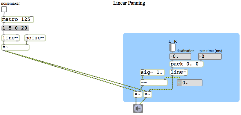
The simplest and most common way to localize a sound in a stereo field is to vary the relative intensity between the two speakers. To make a sound seem to move from one side to the other, for example, you can start with the level of one speaker set to 1 and the other speaker set to 0, then gradually turn one down to 0 as you bring the other up to 1. This patch demonstrates a direct linear pan from one speaker to the other.
The left side of the patch is just a noisemaker, to give us a sound to pan. It creates 8 short bursts of white noise per second. The right side of the patch performs the linear intensity pan. It uses a line~ object to go from 0 to 1 (or 1 to 0) in a given amount of time. (The L-R switch to go from 0 to 1 or 1 to 0 is just a slider object set to have only two possible values.) The value of the line~ object is used directly to control the amplitude of the right speaker, and it is subtracted from a constant signal of 1 to create the opposite amplitude (i.e., 1 minus the amplitude of the right speaker) for the left speaker.
When the panning is at the midway point, both speakers will have an amplitude setting of 0.5 (i.e. -6 dB); but two speakers at -6 dB generally does not produce the same perceived loudness as one speaker at 0 dB. Therefore, this sort of linear amplitude panning creates a slightly lower perceived intensity in the middle than when the sound is panned fully to one side or the other. Because the intensity is lower in the middle, the impression it gives it that the sound is moving slightly farther away from the listener as it moves toward the center location. This is considered to be undesirable in most cases, so panning algorithms often compensate for this effect by increasing the amplitude by about 3 dB as the panning moves to the center position, as demonstrated in the next example.
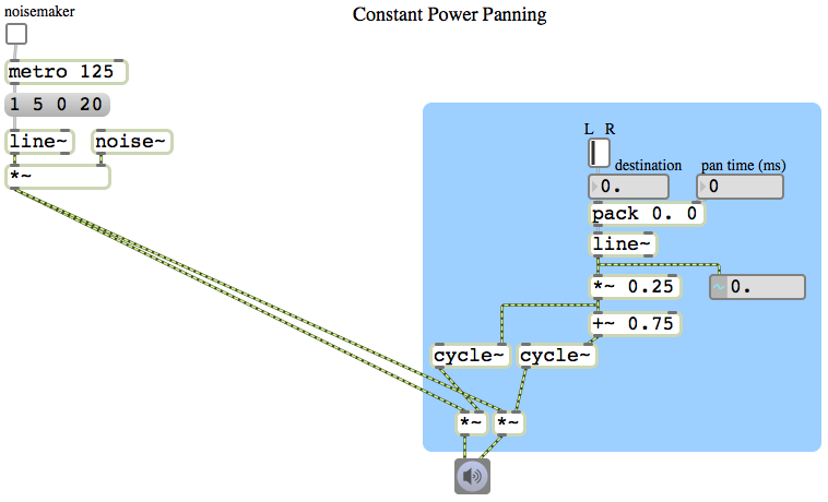
Example 13: Constant power panning using square root of intensity
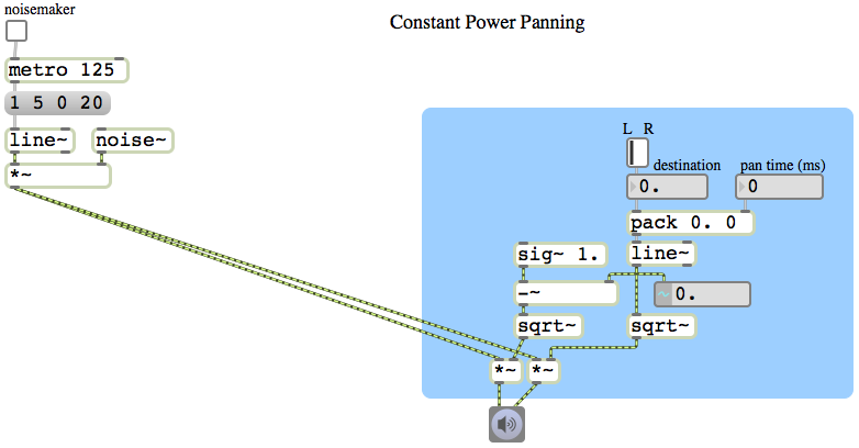
The intensity of sound is proportional to the square of its amplitude. So if we want to have a linear change in intensity as we go from 0 to 1 or 1 to 0, we need to use the square root of that linear change to calculate the amplitude. This example patch is exactly like the previous example, except that we consider the linearly changing signal from line~ to be the intensity rather than the amplitude, and we take the square root of that value to obtain the actual amplitude for each speaker. By this method, when the sound is panned in the center between the two speakers, instead of the amplitude of each speaker being 0.5, it will be the square root of 0.5, which is 0.707 (which is an increase of 3 dB compared to 0.5). This compensates for, and effectively eliminates, the undesirable 'hole-in-the-middle' effect discussed in the previous example.
Example 14: Constant power panning using table lookup
In the previous example we used the square root of the desired intensity for each speaker to calculate the amplitude of each speaker. However, square root calculations are somewhat computationally intensive, and it would be nice if we could somehow avoid having to perform two such calculations for every single audio sample. As it happens, the sum of the squares of sine and cosine functions also equals 1. So, instead of using the square roots of numbers from 0 to 1 (and their complements) to calculate the amplitude for each speaker, we can just look up the sine and cosine as an angle goes from 0 to π/2 (the first quarter of the cosine and sine functions).
In this patch, therefore, we scale the panning value down to a range from 0 to 0.25 and we use that as the phase offset in a 0 Hz cycle~ object. As the panning value moves from 0 to 1, the left speaker's amplitude is looked up in the first quarter of a cosine function and the right speaker's amplitude is looked up in the first quarter of a sine function (by adding an additional 0.75 to the scaled phase offset). The resulting effect is just the same as if we performed the square root calculation, but is less computationally expensive.
In most cases this is the preferred method of constant-power intensity panning between stereo speakers. It's so generally useful that it's worthwhile to implement it and save it as an abstraction, for use as a subpatch in any MSP program for which stereo panning is required. An abstraction version of this method is demonstrated in Example 43 from the 2009 class.
February 23, 2012
Example 15: Getting a sound sample from RAM
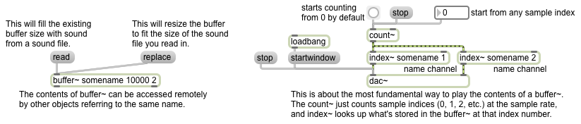
The buffer~ object holds audio data in RAM as an array of 32-bit floating point numbers (floats). The fact that the sound is loaded into RAM, rather than read continuously off the hard drive as the sfplay~ object does, means that it can be accessed quickly and in various ways, for diverse audio effects (including normal playback).
Every buffer~ must have a unique name as its first argument; other objects can access the contents of the buffer~ just by referring to that name. The next (optional) arguments are the size of the buffer (stated in terms of the number of milliseconds of sound to be held there) and the number of channels (1 for mono, 2 for stereo). If those optional arguments are present, they will be used to limit the amount of sound that can be stored in that buffer~ when you load sound into the buffer~ from a file with the 'read' message. If those arguments are absent, when you load in a sound from a file with the 'read' message the buffer~ will be resized to to hold the entire file. The 'replace' message is like 'read' except that it will always resize the buffer~ regardless of the arguments.
The most basic way to use a buffer is simply to access each individual sample by incrementing through the array indices at the sample rate. To do that, the best objects to use are count~, which puts out a signal that increments by one for each sample, and index~, which refers to the buffer~'s contents by the sample index received from count~ and sends that out its outlet. This is good for basic playback with no speed change, or for when you want to access a particular sample within the buffer~.
When count~ receives a 'bang', it begins outputting an incrementing signal, starting from 0 by default. You can cause it to start counting from some other starting sample number by sending a number in its left inlet. (You can also cause it to count in a loop by giving it both a starting and ending number. It will count from the starting number up to one less than the ending number, then will loop back to the starting number.)
Example 16: Simple wavetable synthesis
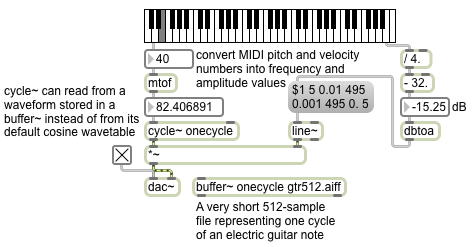
One of the earliest methods of digital sound synthesis was a digital version of the electronic oscillator, which was the most common sound generator in analog synthesizers. The method used was simply to read repeatedly, at the established sample rate, through a stored array of samples that represent one cycle of the desired sound wave. By changing the step size with which one increments through the stored wavetable, one can alter the number of cycles one completes per second, which will determine the perceived fundamental frequency of the resulting tone. For example, if the sample rate (R) is 44100 and the length of the wavetable (L) is 1000 samples, and our increment step size (I) is an expected normal step of 1, the resulting frequency (F) will be F=IR/L which is 44.1 Hz. If we wanted to get a different value for F, while keeping R and L constant, we can just change I, the step size. For example, if we use an increment of 2, leaping over every other sample, we'd get through the table 88.2 times in one second. Thus, by changing I, we can get a cyclic tone of any frequency, and it will have the shape of the waveform stored in the wavetable. (When I is a non-integer number, it will result in trying to read samples at non-existent fractional indices in the wavetable. In those cases, some form of interpolation between adjacent samples is used to get the output value.)
When a cycle~ object refers to a buffer~ by name, it uses the first 512 samples of that buffer~ as its waveform, instead of using its default cosine waveform. In this example, the buffer~ is loaded with a 512-sample file that is actually a single cycle of an electric guitar note. (The file is in the Applications/Max6/patches/docs/tutorial-patchers/msp-tut/ folder of your hard drive, which is probably already included in your file search path, so it should load in automatically.) The frequency value supplied in the left inlet of cycle~ determines the increment I value that cycle~ will use to read through that wavetable. So for this example, we use a MIDI-type pitch number from the left outlet of the kslider and convert it to frequency with the mtof object (which uses a formula such as [expr 440.*pow(2.\,($f1-69.)/12.)] to convert from MIDI pitch number to frequency in Hz). We also use the MIDI-type "velocity" value from the kslider to determine the amplitude of the sound. The velocity value is scaled and offset to give a decibel range between -32 dB and 0 dB; that is used as the peak (attack) amplitude in an amplitude envelope sent to the line~ object to control the amplitude of the cycle~. The amplitude envelope goes to the peak amplitude in 5 ms, then falls to 0.01 (-40 dB) in 495 ms, then falls further to 0.001 (-60 dB) in 495 more ms, and finally goes to 0. (-infinity dB) in 5 ms; so the whole envelope shapes a 1-second note.
Notice that when you play high notes on the keyboard, the tone becomes inharmonic. That's because the stored waveform in the buffer~ is so jagged and creates so many harmonics of the fundamental pitch. When the fundamental is high (in the top octave of this keyboard the fundamental frequencies are all above 1000 Hz) upper harmonics of the tone get folded back due to aliasing, resulting in pitches that don't belong to the harmonic series of the fundamental.
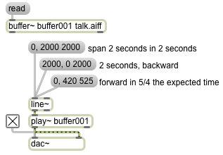
Example 17: Playing a sample from RAM
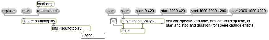
You can use the play~ object to play the contents of a buffer~, simply by sending it a 'start' message. By default it starts from the beginning of the buffer~. You can specify a different starting time, in milliseconds, as an argument to the 'start' message, or you can specify both a starting time and a stopping time (in ms) as two arguments to the 'start' message. In the patch, you can see two examples of the use of starttime and stoptime arguments. The message 'start 0 420' reads from time 0 to time 420 ms, then stops. You can cause reverse playback just by specifying a stop time that's less than the start time; the message 'start 2000 420' starts at time 2000 ms and plays backward to time 420 ms and stops. In all of these cases -- start with no arguments, start with one argument, or start with two arguments -- play~ plays at normal speed. If you include a third argument in the 'start' message, that's the amount of time you want play~ to take to get to its destination; in that way, you can cause play~ to play at a different rate, just by specifying an amount of time that's not the same as the absolute difference between the starttime and stoptime arguments. For example, the message 'start 1000 2000 1200' means "play from time 1000 ms to time 2000 ms in 1200 ms." Since that will cause the playback to take 6/5 as long as normal playback, the rate of playback will be 5/6 of normal, and thus will sound a minor third lower than normal. (The ratio between the 5th and 6th partials of the harmonic series is a pitch interval of a minor third.) The message 'start 2000 1000 4000' will read backward from 2000 ms to 1000 ms in 4000 ms, thus playing backward at 1/4 the original rate, causing extreme slowing and a pitch transposition of two octaves down.
The info~ object, when it receives a bang in its inlet, provides information about the contents of a buffer~ object. Since the buffer~ object sends a bang out its right outlet when it has finished a 'read' or 'replace' operation, we can use that bang to get information about the sound that has just been loaded in. In this example, we see the length of the buffer, in milliseconds. You can use that information in other parts of your patch.
Example 18: Sample playback driven by a signal
The play~ object can be controlled by any MSP signal in its inlet. The value of the signal controls the location in the buffer~, in milliseconds. Normal playback can be achieved in this way by using a linear signal, such as from a line~ object, that traverses a given time span in the expected amount of time. By making a signal that goes linearly from a starttime to a stoptime in a certain amount of time, line~ can be used to get the same sorts of playback as with the 'start' message with three arguments demonstrated in the previous example.
In this patch you can see how the line~ object is commanded to leap to a particular value, then proceed to a new value linearly in a certain amount of time. The existence of a comma in a message box divides the message into two separate messages, sent out in succession as quickly as possible. So a message such as '0, 2000 2000' sends out the int message '0' followed immediately by the list message '2000 2000'. The int causes line~ to go to the value immediately, and the list causes line~ to use the number pair(s) as destination and ramptime. So the first message says, "Go to 0 immediately, then proceed toward 2000 in 2000 milliseconds." This will result in normal forward playback. Going from 2000 to 0 in 2000 milliseconds causes backward playback at normal speed. Going from 0 to 420 in 525 milliseconds causes the playback to be at 4/5 normal speed, which also causes downward transposition by a major third.
Example 19: DJ-like sample scrubbing
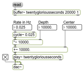
Although playback is normally achieved by progressing linearly through a stored sound, other ways of traversing the sound can give interesting results. Moving quickly back and forth in the sound is analogous to the type of "scrubbing" achieved by rocking the reels of a tape recorder back and forth by hand, or by "scratching" an LP back and forth by hand. In this example, we use a cycle~ object to simulate this sort of scrubbing. The output of cycle~ is normally in the range -1 to 1, so if we want its output to be used as the playback position in milliseconds, we need to scale its output with a *~ object and offset it with a +~; the multiplication will determine the depth (range) of the scrubbing, and the addition will determine the center time around which the scrubbing takes place. Initially the patch is set to scrub the entire range of the buffer~ in a time span (period) of 40 seconds. You can get different results by changing, in particular, the rate and depth values. For example, with a depth of about 250 milliseconds and a rate of about 3 Hz, you can get a sound that's much more like tape reel scrubbing or LP scratching.
Example 20: Playing a sample with groove~
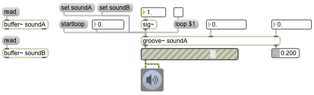
The groove~ object plays sound from a buffer~, using two important pieces of information: a rate provided as a MSP signal and a starting point provided as a float or int message. For normal playback, the rate should be a signal with a constant value of 1. (The sig~ object is a good way to get a constant signal value.) A rate of 2 will play at double speed, a rate of 0.5 will play at half speed, and so on. Negative rate values will play backward. The starting point is stated in milliseconds from the beginning of the buffer~. In the example patch, read some sound into the buffer~ objects, turn up the gain~, send a starting point number to groove~'s left inlet from the number box, and set the sig~ value to 1. The sound will play till the end of the buffer~ is reached or until the rate is set to 0 (or until a new starting point is sent in the left inlet.)
You can use a 'set' message to groove~ to cause it to access a different buffer~. All its other settings will stay the same, but it will simply look at the new buffer~ for its sample data. You can test this by clicking on the 'set soundA' and 'set soundB' message boxes.
One of the important features of groove~ is that it can be set to loop repeatedly through a certain segment of the buffer~. You set groove~'s loop start and end times (in ms) with numbers in the second and third inlets. By default, looping is turned off in groove~, but if you send it a 'loop 1' message it will play till the loop end point, then leap back to the loop start point and continue playing. When looping is turned off, the loop end point will be ignored and groove~ will play till the end of the buffer~. To loop the entire buffer~, set the loop start and end times to 0. (An end time of 0 is a code to groove~ meaning "the end of the buffer~".)
You can also cause groove~ to start playing from the loop start time with the 'startloop' message. This works even when looping is turned off, but the loop end point will be ignored if looping is turned off. (Note that 'startloop' does not mean "turn looping on"; it means "start playing from whatever time is set as the loop start time".)
Whenever groove~ leaps to a new point in the buffer~ -- either because of a float or int message in its left inlet, or with a 'startloop' message, or by reaching its loop end time and leaping back to the loop start time -- there is a potential to cause a click because of a sudden discontinuity in the sound. Tha potential problem is addressed in the next few examples.
Example 21: Random access of a sound sample
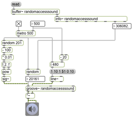
The fact that groove~ can leap to any point in the buffer~ makes it a suitable object for certain kinds of algorithmic fragmented sound playback. In this example it periodically plays a small chunk of sound chosen at random (and with a randomly chosen rate of playback).
The info~ object reports the length of the sound that has been read into the buffer~, and that number is used to set the maximum value for the random object that will be used to choose time locations. When the metro is turned on, its bangs trigger three things: an amplitude envelope, a starting point in ms, and a playback rate. The starting point is some randomly chosen millisecond time in the buffer~. The rate is calculated by choosing a random number from 0 to 200, offsetting it and scaling it so that it is in the range -1 to 1, and using that number as the exponent for a power of 2. That's converted into a signal by the sig~ object to control the rate of groove~. (2 to the -1 power is 0.5, 2 to the 0 power is 1, and 2 to the 1 power is 2, so the rate will always be some value distributed exponentially between 0.5 and 2.)
The amplitude envelope is important to prevent clicks when groove~ leaps to a new location in the buffer~. The line~ object creates a trapezoidal envelope that is the same duration as the chunk of sound being played. It ramps up to 1 in 10 milliseconds, stays at 1 for some amount of time (the length of the note minus the time needed for the attack and release portions), and ramps back to 0 in 10 ms. Notice that whenever the interval of the metro is changed, that interval minus 20 is stored and is used as the sustain time for subsequent notes. This pretty effectively creates a trapezoidal "window" that fades the sound down to 0 just before a new start time is chosen, then fades it back up to 1 at the time the new note is played.
MSP calculates audio signals several samples at a time, in order to ensure that it always has enough audio to play without ever running out (which would cause clicks). The number of samples it calculates at a time is determined by the signal vector size, which can be set in the Audio Status window. If the sample rate is 44100 Hz, and the signal vector size is 64, this means that audio is computed in chunks of 1.45 ms at a time; a larger signal vector size such as 512 would mean that audio is computed in chunks of 11.61 ms at a time. For this reason, the millisecond scheduler of Max messages might not be in perfect synchrony with the MSP calculation interval based on the signal vector size. This causes the possibility that we will get clicks even if we are trying to make Max messages occur only at moments when the signal is at 0. For that reason, you need to be very careful to synchronize those events carefully. One thing that can help is to synchronize the Max scheduler to send messages only at the same time as the beginning of a signal vector calculation. You can do that by setting the Scheduler in Overdrive and Scheduler in Audio Interrupt options both On in the Audio Status window. Another useful technique (although not so appropriate with groove~, which can only have its starting points triggered by Max messages) is to cause everything in your MSP computations to be triggered by other signals instead of by Max messages. This will be demonstrated in the next few examples.
Example 22: The phasor~ object
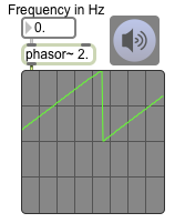
The phasor~ object is one of the most valuable MSP signals to use as a control signal. (You wouldn't generally want to listen to it directly as audio because it's an ideal sawtooth wave and has energy at so many harmonics that it can easily create aliasing. If you want a sawtooth wave sound, it's better to use the saw~ object, which limits its harmonics so as not to exceed the Nyquist frequency.) The phasor~ outputs a signal that ramps cyclically from 0 to 1. It's actually more correct to say that phasor~ ramps from 0 to almost 1, because it will never actually output the value 1; it will instead output 0 because the end of a ramp is the same moment as the beginning of the next ramp. Because phasor~ is constantly moving and interpolating between 0 and 1, it's usually best not to rely on detecting any specific value in its output signal, but just to know that it's always increasing linearly from 0 toward 1.
This patch simply allows you to see the signal produced by phasor~. The next four examples show some ways it can be useful.
Example 23: Using phasor directly as a control signal
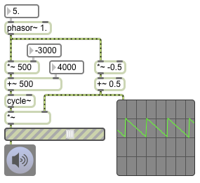
If you need a linear signal that repeats at a specific rate, phasor~ can be scaled and offset to provide a repeating line from one signal value to another. In this example, we use phasor~ to directly control both frequency and amplitude of an oscillator.
Since phasor~ ramps from 0 to (almost) 1, it would normally create a crescendo in amplitude, and indeed it can be useful for that purpose over long periods of time as a control signal for other control signals. A more normal amplitude envelope for a single note, however, goes quickly to a peak amplitude and then gradually decreases to 0 over the course of the note. So in this patch we multiply the phasor~ signal by -0.5, which causes it to ramp from 0 to -0.5, and then we add 0.5 to that so that it is now ramping from 0.5 to 0. (Notice that the leap up from 0 to 0.5 is instantaneous, though, causing a click in this case. A more sophisticated program might do something to smooth that transition.) We use a similar scaling and offsetting procedure for the control of frequency of the cycle~. We multiply the phasor~'s output by 500 then add 500 to that so that the result is a ramp that goes from 500 to 1000 (a number that we use as Hz in the cycle~). You can experiment with other rate settings for the phasor~ and other frequency ranges for the cycle~.
Example 24: Repeatedly reading a function with phasor~
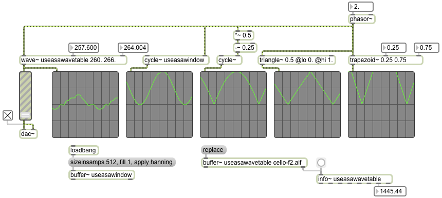
The real value of phasor~ is that it provides a very accurate way to read through (or mathematically calculate) some nonlinear shape to use as a control signal (or even as an audio signal). Among other things, it might be used to create a "window" shape that can serve as an amplitude envelope for a sound. This patch demonstrates five different ways to create window or waveform shapes with phasor~. We'll discuss them (in good Max fashion) from right to left.
The trapezoid~ object expects a signal that progresses from 0 to 1. It has two arguments (or values it can receive): one to say at what point its upward ramp should end, and the other to say at what point its downward ramp should begin. So in this example, as the phasor~ signal goes from 0 to 1, the trapezoid~ object will ramp upward and arrive at 1 just as phasor~ gets to 0.25 (the first argument of trapezoid~), then trapezoid~ will stay at 1 till phasor~ gets to 0.75 (the second argument of trapezoid~) at which point trapezoid~ will begin to ramp back down to 0 and will arrive there just as phasor~ completes its cycle. This can be useful for tapering the ends of some other signal (such as notes or loops played by a groove~ object) to avoid clicks.
The triangle~ object similarly makes a simple shape when driven by a signal between 0 and 1. The first argument of triangle~ specifies where in the phasor~'s 0-to-1 range the highpoint of the triangle should occur, and the lo and hi attributes specify the minimum and maximum output values.
The output of phasor~ can be used to control the phase offset of a cycle~ object (in cycle~'s right inlet). If the cycle~'s frequency is 0, the signal from phasor~ will specify the exact location (on a scale from 0 to 1) in the wavetable that cycle~ will send out. Since cycle~ uses a cosine wavetable by default, scanning through the entire wavetable (0 to 1) in this way would cause cycle~ to output a cosine wave. However, in this example we scale and offset the phasor~ signal so that it goes cyclically from -0.25 to 0.25, thus cycling through the first half of a sine wave. This creates a window shape that's commonly called a cosine window, which is also useful as an amplitude envelope, particularly for short notes.
Because the cycle~ object can use a buffer~ as a wavetable (see Example 16 above), we can fill a buffer~ with 512 samples of any shape we want, and then read through that function with cycle~. The buffer~ object even has a few messages for doing just that. In this patch we have created a buffer~ called "useasawindow", we set its size to 512 samples, we fill it with all values of 1, and then we impose a "hanning" (or "Hann") window on it. (A hanning window is really just cosine waveform that has been scaled and offset.)
The wave~ object can also access samples in a buffer~ in a fashion similar to a cycle~ (with frequency 0) driven by a phasor~. A difference with wave~ is that it can use any portion of a buffer~ as its wavetable. You specify the start and end points (in ms) of the portion of the buffer that you want to use, and wave~ will use that as its wavetable to read when it is driven by a signal from 0 to 1. In this patch we use a small portion (about one cycle) of a cello note. When phasor~ is at a very low subaudio frequency (such as 1 Hz.) you can see the waveform pretty clearly in the scope~. To hear it, raise the phasor~ to an audio frequency (and turn up the gain~). As you change the range of the buffer~ that is being accessed by wave~, the timbre of the tone will change (because the resulting waveform is changing), but the fundamental frequency of the wave is still largely determined by the rate of the phasor~.
Example 25: Triggering events with each cycle of a phasor
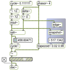
How do we detect, with sample-accurate precision, the precise moment when phasor~ begins a new cycle from 0 to 1? We need to detect the sample on which it leaps from 1 back to 0. However, because phasor~ is constantly interpolating between 0 and 1, it might not leap down to exactly 0. So we can't just use a ==~ object to see when its value is 0. Its exact value is relatively unknowable with any great precision; all we know is that it's always increasing...except at the one instant when it leaps back down to (approximately) 0 and begins again. However, that instant is so remarkable that there is a way to detect it, with the help of an object called delta~. A delta~ object sends out a signal in which each sample reports the change in its input relative to the previous sample. So, if we send a phasor~ into a delta~, delta~ will always report a positive increase (or 0 if the phasor~ is completely stopped), except for when the phasor~ leaps downward. That's the one sample on which delta~ will report a negative value. So we can use a <~ 0 object to detect the sample on which that occurs. The <~ 0 object will always output a signal of 0 (false) except for that one sample when it will report a 1 (true).
The sah~ object implements a "sample-and-hold" mechanism. When a particular threshold is surpassed in the signal in its right inlet, it will sample the value of the signal in its left inlet and will hold that as a constant output signal value until the next time the threshold is surpassed in the right inlet. By default its threshold is 0, so every time the <0~ object sends out a 1 preceded by a 0 it will cause sah~ to sample its left input. We use that fact to sample the slowly moving sinusoidal control value coming from cycle~ via mtof~. The cycle~ is moving slowing with a period of 9 seconds, and it's varying + or - 12 semitones from a central pitch of 72 (C above middle C); that signal value is converted to frequency by the mtof~ (MIDI to frequency) object and that is sampled and held 4 times per second by the sah~ which is triggered by the phasor~. That frequency value from sah~ -- which is constant for each 1/4 second until it is changed by sah~ -- is used by cycle~ as its frequency value for its notes.
The individual notes are shaped by a trapezoidal amplitude envelope. The envelope is almost rectangular, but it has a very quick ramp up and down during the first and last 2% of each note (5 ms in this case). Because the change in frequency of the cycle~ that we're listening to is triggered by the beginning of each cycle~ of the phasor~, it's perfectly synchronized with the trapezoidal amplitude envelope.
If you want to use the beginning of a phasor~ ramp to trigger events in other parts of a Max patch, you can use an edge~ object to detect the 1 values coming from the <~ 0 object. The edge~ will send out a bang when a 0-to-1 or 1-to-0 transition occurs in a signal vector. But it can only do so with as much precision as the Max scheduler provides, which is not sample-accurate. So in this patch we use edge~ to detect the 0-to-1 transitions, then we use that bang to trigger a report of the current frequency value with a snapshot~ object. Note that not only will the edge~ object not send a bang with sample-rate precision, snapshot~ will only report the value at the beginning of the signal vector when (or immediately after) it receives the bang. So these translations between the sample-accurate-but-vector-based timing of MSP and the millisecond (or vector-based) timing of the Max scheduler show the slight difference between the true sample-accurate timing of the phasor~ and the close approximation that we can achieve with edge~. When you stop the audio (by turning off the dac~), you will probably notice a slight difference between the actual frequency being reported by the number~ object and the frequency reported by snapshot~ at the beginning of the vector when it was triggered by edge~. In many cases this difference is negligible, but in some cases it can lead to clicks when sudden changes are made in an audio signal that is not at 0 amplitude.
Example 26: Transport-controlled phasor~
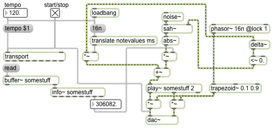
A phasor~ object, like other MSP objects such as cycle~ that use a rate for their timing, can have its repetition rate specified as a transport-related tempo-relative time value (note values, ticks, etc.). So if you want a phasor~ to work at a rate that is related to the transport's tempo, you can type in a tempo-relative time as an argument to specify its period of repetition instead of typing in a frequency. The existence of that time syntax argument will tell the object to use the transport's tempo as its basis of timing. MSP objects that are using transport-based timing will work -- and will respond to changes in the transport's tempo -- even when the transport is not turned on. By setting the object's 'lock' attribute to 1, you can cause the object to sync precisely to the quantized note value of the moving transport. When the lock attribute is on, the object will only work when the transport is on.
In this example we have a phasor~ with a typed-in argument of 16n and a lock attribute setting of 1. This means that it will only move forward when the transport is running, and its period of repetition will be synchronized with the 16th notes of the transport.
Read some sound into the buffer~. This will cause the length of the sound file to go to the right inlet of the *~ object. The noise~ object generates random sample values in the range -1 to 1. We use the sample-and-hold trick that was explained in Example 25 to get individual random numbers at a time that's perfectly synchronized with the start of each phasor~ cycle, we take the absolute value of that (to force the number to be positive) scale it to be a useful time value within the buffer~, and use that as a starting point for play~ each time the phasor~ starts a new ramp. By translating the 16th-note note value into milliseconds, we can scale the phasor~ ramp to traverse one 16th note's worth of time in the play~ object, offset by the starting point we got from sah~. The same phasor~ is used to make a trapezoidal amplitude envelope for each 16-note chunk of audio we play. The result is randomly-chosen 16th-note soundbites played continuously and in synchrony with the transport (and click-free) from the buffer~.
February 28, 2012
Example 27: Simple delay of audio signal
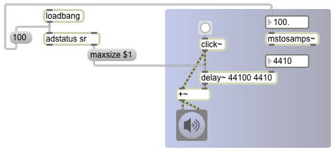
The delay~ object creates a "ring buffer" into which it constantly records the signal coming in its left inlet. The first typed-in argument specifies the size of the buffer, in samples. The second argument (or a number in the right inlet) specifies how many samples in the past delay~ should look for the signal it will send out its outlet. So, assuming a sample rate of 44100 Hz, this patch creates a one-second buffer and instructs delay~ to send out the sound it received 1/10 of a second ago.
Entering those values as typed-in arguments makes a rather unsafe assumption about the sample rate. (The sample rate could be 48000 or 96000 or whatever the user has set it to.) A better way to make sure you're allotting the correct amount of memory and specifying the correct delay time is to use an [adstatus sr] object (which can be triggered by loadbang to report the sample rate) to calculate the size of the buffer in samples (in this case we know we want 1 second's worth of memory, so we can use the sample rate directly), and use the mstosamps~ object (which will make its calculation based on the current sample rate) to convert the desired delay time from milliseconds to samples.
When the click~ object receives a bang it sends out a single sample with a value of 1; it sends out all 0 values otherwise. That's a very clearly defined moment in time (known as an "impulse") that lets you confirm that delay~ is doing what it's supposed to do.
Example 28: Delay with tempo-relative timing
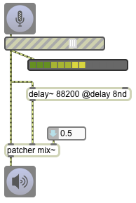
The delay attribute (the delay time) of a delay object can be specified with tempo-relative timing (such as notevalues) instead of samples. This example shows a delay time of a dotted eighth note rhythmic value, at whatever the current transport tempo is. The transport tempo is 120 bpm by default; a dotted eighth note at that tempo will last 375 ms which, at a sample rate of 44100 samples per second, is 16,537.5 samples. Specifying the delay time as a rhythmic value allows you not to have to worry about the math of exactly how many samples of delay you need (other than making sure that you create a big enough buffer for delay~). In this case, 88200 samples' worth of memory space will be a great plenty for a dotted eighth note at any reasonable tempo.
This example shows the use of a gain~ object so that we can control the level of sound that is coming into MSP from the audio input (which allows us to turn the audio input down to 0 if we need to do so), and a meter~ object to show how much signal is being sent to delay~. There is also a subpatch that allows you to control the balance between direct input sound and delayed sound. The right inlet of the subpatch expects a value from 0 to 1, where 0 is all direct sound and no delayed sound, a value of 1 is all delayed sound and no direct sound, and a value of 0.5 will be a half-and-half mix of the two. In audio processing terminology this value is often referred to as the "wetness" or the "wet/dry mix", meaning the balance between the effect and the original sound. (Double click on the patcher object to see its contents.) This kind of simple mixer is frequently useful when applying audio effects.
Example 29: Ducking when changing delay time
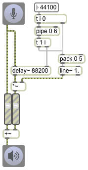
Whenever you change the delay time, you're asking MSP to look at a new location in the delay buffer, which can cause a click in the output if the new sample value is very different from the previous one. One way to get around that is to quickly fade the output amplitude down to 0 whenever you make a change, then quickly fade it back up once the change has been made. In this example, whenever a new delay time comes out of the number box, it first sends a 0 to the pack object, which sends a '0 5' message to line~, which fades line~'s signal down to 0 in 5 milliseconds (meaning the output signal of delay~ will get multiplied by 0, silencing it). The delay time meanwhile is held for 6 milliseconds by the pipe object, thus waiting for the fade-down to be completed by line~. Only then does the new delay time get passed on to the delay~ object, and then a 1 gets sent to pack, sending a '1 5' message to line~, fading the sound back up in 5 ms. The net effect is that we do get a very quick (11-ms) fadedown/fadeup in the output of delay~, but at least it's not a jarring click.
Example 30: Simple flanging
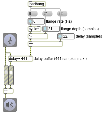
The number of samples of delay can be provided in the right inlet of delay~ as a MSP signal instead of an individual Max int message. The main reason for doing that would be to get a special effect by continuously modulating the delay time. When the delay time is continuously modulated by a repeating signal such as a low-frequency oscillator (LFO), the effect is called "flanging". (Essentially, any time the delay is changing continuously, that's a simulation of the sound source moving toward us or away from us, which introduces a "Doppler shift" in the perceived pitch.) Notice that the signal in the right inlet of delay still represents samples of delay, so we need to scale the output of cycle~ to the appropriate range and offset its center point. In this example we scale its range to + or - 21 samples and offset that by 22 samples, so the delay time fluctuates between 1 and 43 samples, 6 times per second. Subtle flanging of + or - 1/2 ms, as is shown in this example, imposes a modest vibrato on the incoming sound. You can play around with different flange rates and different depths of vibrato to get a variety of effects. When the flanged sound is mixed with the direct sound, the two sounds interfere in potentially interesting ways.
Example 31: Delay with feedback
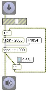
The delay~ object does not permit its delayed signal to be fed back into its own left inlet. (You can probably imagine how that would make it impossible for MSP to calculate the correct signal, since you'd be asking it to perform infinite recursion: the signal plus the delayed signal plus the delayed sum of those two plus...). If you want to get delay with feedback, you need to use objects that are designed to handle that.
The tapin~ and tapout~ objects together work similarly to the delay~ object. The tapin~ object allows you to create a ring buffer containing the most recently received signal, and you specify the size of the buffer as the argument to tapin~ -- in terms of milliseconds. (The size in samples will be calculated automatically based on the sample rate.) A tapout~ object that's connected to the tapin~ object will refer to that ring buffer and will look a certain amount of time in the past for its output (whatever number of milliseconds you specify). In this case we typed in 1000 ms as the delay time for tapout~ to use, but that can be changed with a number in the inlet.
Unlike the delay~ object, which can have a delay time as small as one sample, tapout~ has a minimum delay time of one signal vector. (The signal vector size is specified in the Audio Status window.) This might be a disadvantage if you want extremely short delay times (in which case delay~ might be a better object to use), but it has the advantage of permitting its output to be fed back into the inlet of tapin~ (because MSP can calculate each vector's samples without having to account for the delayed sound from the same vector). Feeding the delayed sound back into the delay buffer allows for echos of echos, giving the potential for a series of repeating echos using a single delay tap. But one must be careful not to create a situation in which the sum of the original signal and the delayed signal, plus a delayed version of that, etc., grows ever louder and causes clipping. For that reason, you almost invariably will want to multiply the delayed signal by some number between 0 and 1 to scale down its amplitude.
March 8, 2012
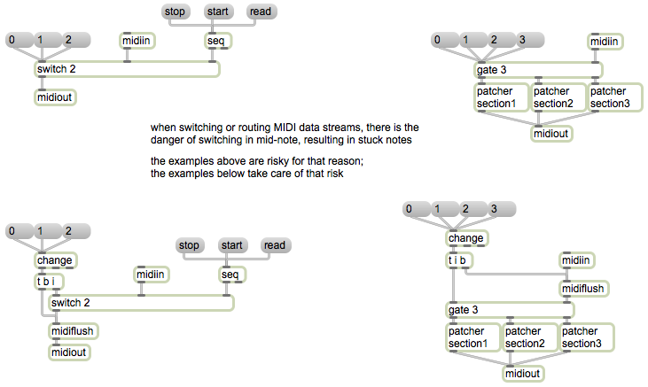
Example 32: Routing MIDI data flow
Managing the flow of data in a program is a common issue. Often you'll want to receive data from different sources, or send it to different destinations.
To receive data from one of multiple sources, the switch object can be used to pass out the messages that come in just one (and only one) of its inlets at a time, ignoring any messages that may be coming in other inlets in the meantime. The leftmost inlet is the control inlet, used to determine which of the other inlets will be "open" and will pass its messages out the outlet. 0 in the control inlet means all inlets are closed; 1 means that the 1st of the other inlets is "open", and so on.
The gate object is a counterpart of switch. Its left inlet is the control inlet, just as with switch. The number received in the left inlet determines which outlet will be "open", and gate will pass messages from its right inlet to that open outlet.
These patches demonstrate how switch and gate can be used to manage the flow of MIDI data in a patch. In the upper left, the switch object allows us to choose which source of MIDI data we want to pay attention to -- the data coming from the midiin object or the data coming from the seq object. In the upper right, a gate object allows us to direct the data from midiin to one of three different subpatches. This potentially allows a single program to process incoming MIDI data in one of several different ways (in different subprograms).
The principle, in each case, is for a single program to be able to do different things, to process information differently, at the flip of a switch.
Notice one little potential problem. If we cut off a flow of MIDI messages, there is always the chance that we might interrupt the flow of data between a note-on message and its corresponding note-off message, resulting in a stuck note. The patches in the lower part of the example demonstrate reasonable precautions to protect against such stuck notes occurring.
The midiflush object is designed to turn off held notes. It keeps track of each MIDI note-on message that passes through it until it receives a corresponding note-off message. Thus, it always has in its memory all the held notes that have not yet been turned off. When it receives a bang, it sends out a note-off message for any remaining note-ons.
In each of the two lower patches, we check to see when the control inlet of the switch or gate object is changed, by using the change object. (There will only be output from the change object when its input actually changes.) When it does change, we send a bang to midiflush to turn off any notes that are held at the moment. Notice that in the patch on the right it's important to send the bang to midiflush before switching the outlet of gate, to make sure that the note-offs go out the proper outlet.
Example 33: Routing audio data flow
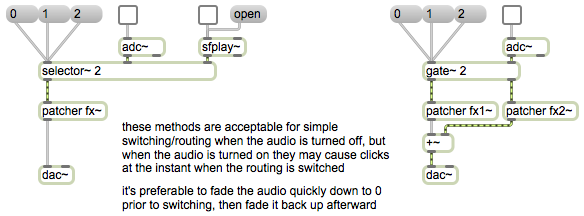
The selector~ and gate~ objects serve the same function for audio signals as the switch and gate objects do for Max messages. The selector~ object chooses one signal inlet to pass to its outlet. The gate~ object chooses one outlet out of which to pass its incoming signal.
Because the selector~ and gate~ objects make their changes instantly, they might cause a click to occur in the audio signal. For this reason, they're best used only for situations when there's no signal passing through them or when the signal is at 0. In general, to make such a switch you'll want to fade the audio signal quickly down to 0 before making the switch, then fade it back up immediately afterward.
Example 34: Smooth audio switching to bypass an audio effect
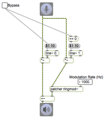
This example shows how, instead of switching instantaneously from one audio signal to another, we can do a quick crossfade between signals, thus avoiding clicks. The patch illustrates a common reason for switching signals -- to bypass an audio effect.
Initially the incoming signal from adc~ goes through a ring modulation supatch. (Notice that the line~ object on the left is initialized to a 0 signal, and the one on the right that's going to the ring modulator is initialized to 1.) If we want to bypass the ring modulation effect, we just click on the toggle, sending a 1 to the left line~ object (thus passing an unchanged signal through the *~ object to the +~ object); however, the 1 from the toggle also goes to the == 0 object (but is not equal to 0), thus sending a 0 to the other line~ object, turning it off. The toggle acts as a bypass switch by quickly crossfading from processed signal to unprocessed signal.
Example 35: Using matrix~ for audio routing and mixing
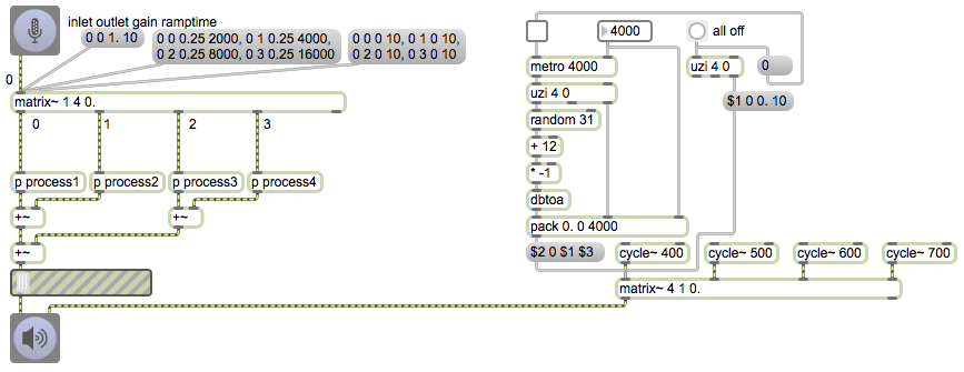
The matrix~ object is an audio mixer/router that can be configured with any number of inlets and outlets. The arguments specify the number of audio inlets, the number of audio outlets (there's always one additional outlet on the right), and the initial gain for the connections of inlets to outlets. Each inlet is potentially connectable to each outlet with a unique gain setting. The gain of the connections is changed by sending messages in the left inlet.
The messages in the left inlet of matrix~ specify an inlet number (numbered starting from 0), an outlet number, a gain factor for scaling the amplitude of that connection, and a ramp time in milliseconds to arrive at that amplitude. You can send as many such messages as needed to establish all the desired connections.
The patch on the left shows how matrix~ can be used to route a signal to multiple destinations. The first message connects inlet 0 to outlet 0 with a gain factor of 1 and a ramp time of 10 milliseconds, which is to say that it quickly opens the first outlet. The next message sets all four outlets to an amplitude of 0.25, but assigns a different fade time to each outlet, which shows that matrix~ can be used as a mixer as well as a simple router. The third message quickly turns off all four outlets (turns them all to 0 amplitude in 10 ms).
This method of sending a message for each possible connection may seem a bit cumbersome, but in fact it's about the most efficient way to control a large matrix (a virtual patchbay) of possible connections. With some clever message management, you can control or automate a great many constantly-changing connections. The patch on the right automates a constantly-changing mix of four sound sources.
Every four seconds (or whatever time interval you choose) the metro bangs an uzi object which outputs four messages (numbers from 0 to 3 out its right outlet, and four bangs out its left outlet), which in turn trigger four messages to matrix~. Each bang from uzi chooses a random amplitude from -12 dB to -42 dB, packs it with a connection number and a transition time, and formats that as a connection message for matrix~.
March 13, 2012
Example 36: Phase cancellation
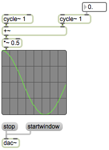
Example 37: Comb filter
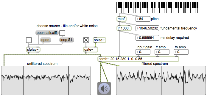
Example 38: The simplest lowpass filter
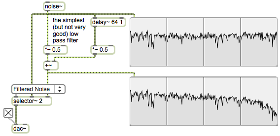
Example 39: Resonant lowpass filter
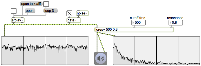
Example 40: Resonant bandpass filter
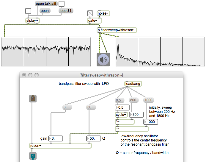
Example 41: Rhythmic filtered noise bursts
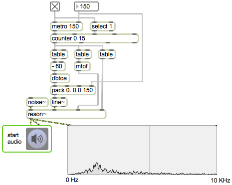
Example 42: ADSR amplitude envelope
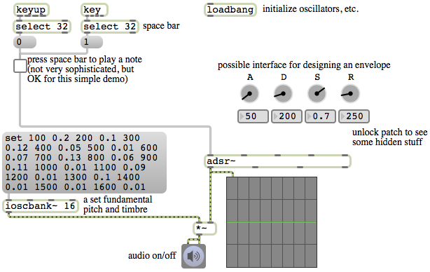
Example 43: ADSR filter envelope
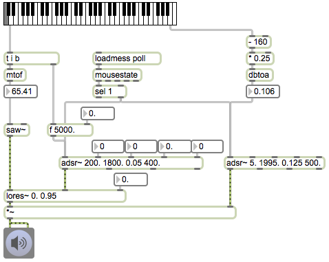
Example 44: Biquad filter
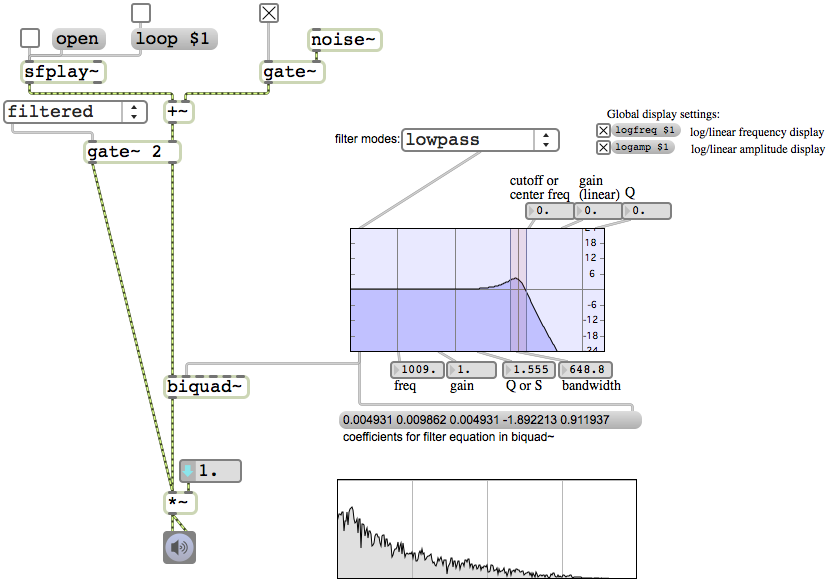
This page was last modified March 14, 2012.
Christopher Dobrian
dobrian@uci.edu